Path Analysis
Path analysis is a type of statistical method to investigate the direct and indirect relationship among a set of exogenous (independent, predictor, input) and endogenous (dependent, output) variables. Path analysis can be viewed as generalization of regression and mediation analysis where multiple input, mediators, and output can be used. The purpose of path analysis is to study relationships among a set of observed variables, e.g., estimate and test direct and indirect effects in a system of regression equations and estimate and test theories about the absence of relationships
Path diagrams
Path analysis is often conducted based on path diagrams. Path diagram represents a model using shapes and paths. For example, the diagram below portrays the multiple regression model $Y=\beta_0 + \beta_X X + \beta_W W + \beta_Z Z + e$.
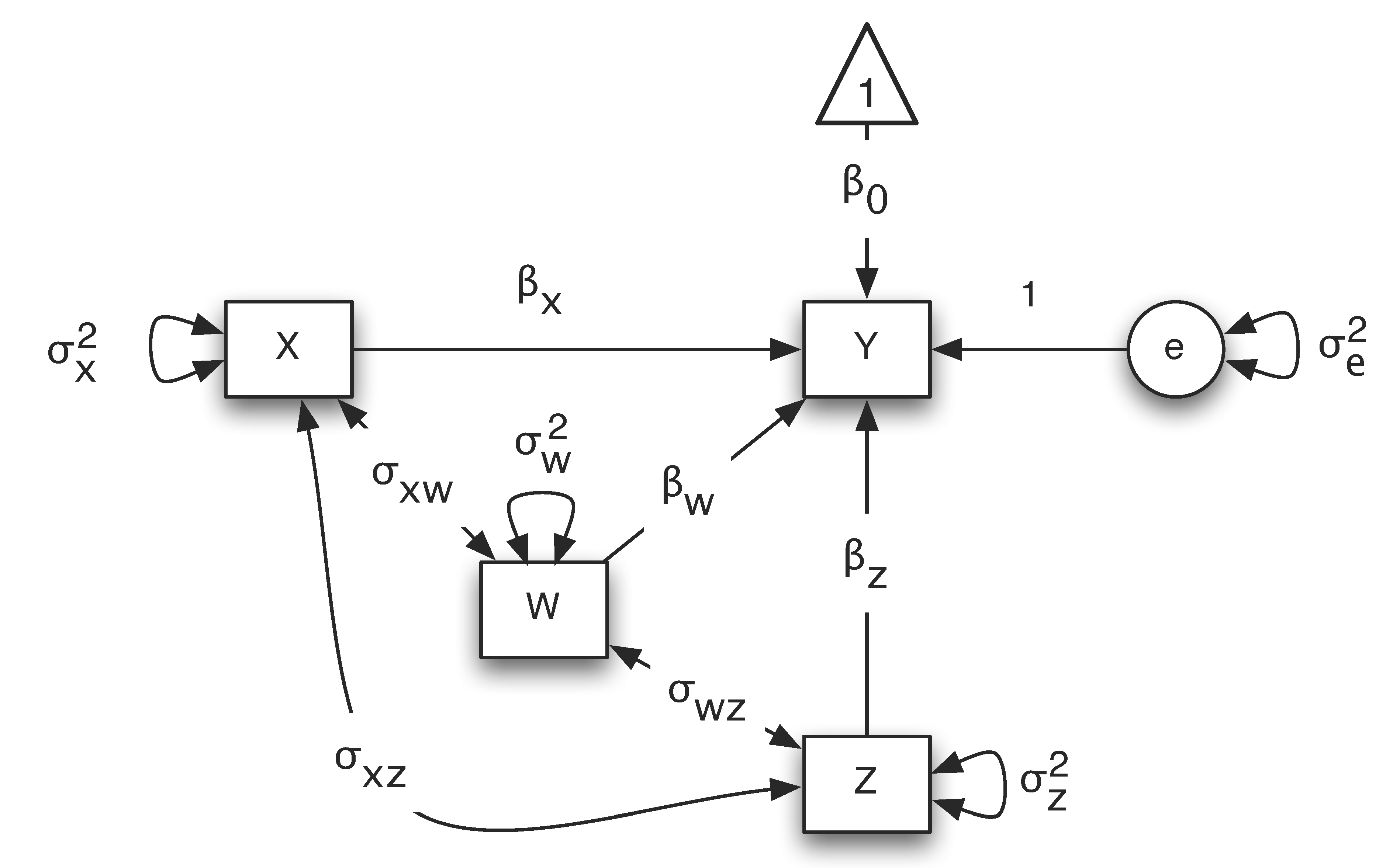
In a path diagram, different shapes and paths have different meanings:
- Squares or rectangular boxes: observed or manifest variables
- Circles or ovals: errors, factors, latent variables
- Single-headed arrows: linear relationship between two variables. Starts from an independent variable and ends on a dependent variable.
- Double-headed arrows: variance of a variable or covariance between two variables
- Triangle: a constant variable, usually a vector of ones
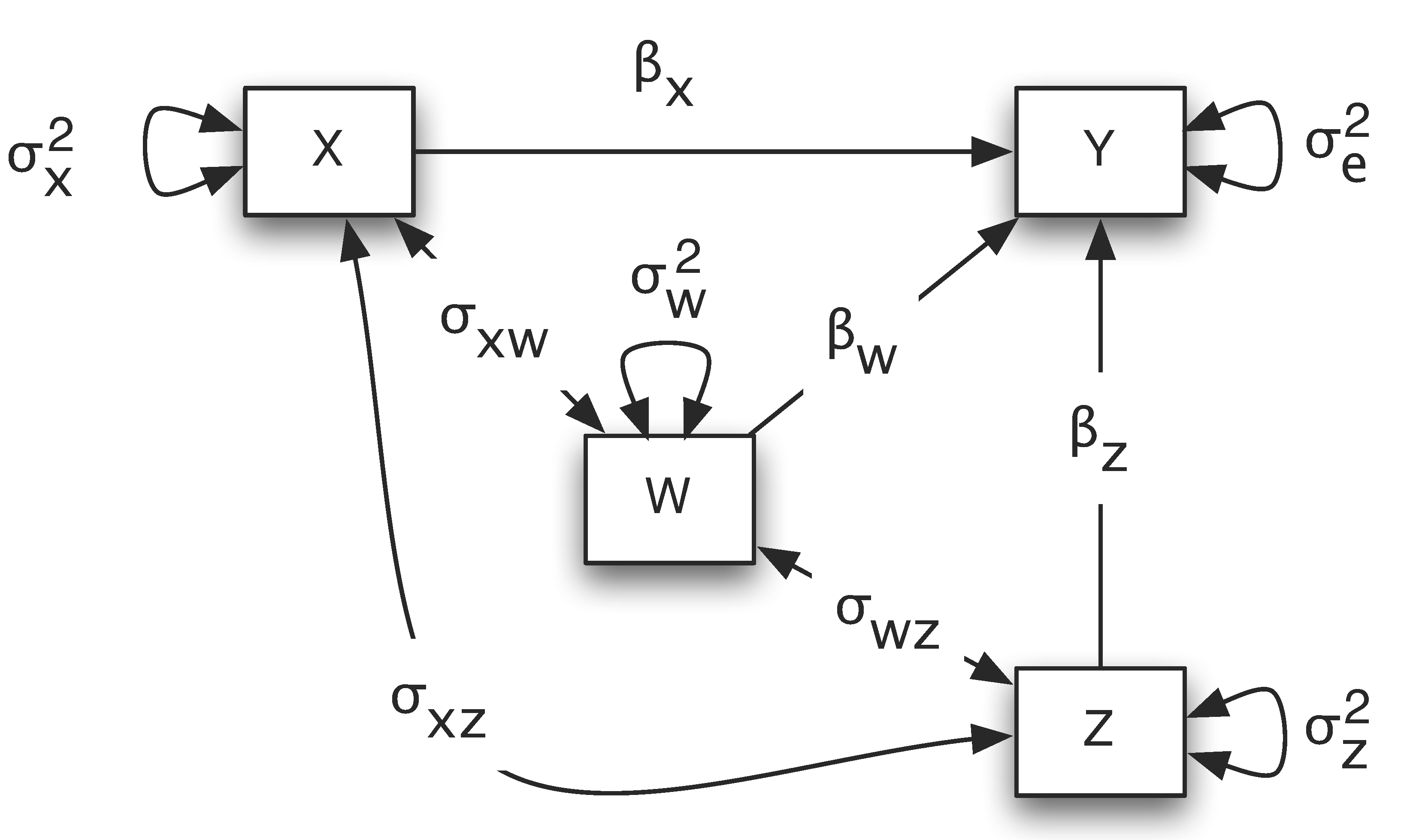
A simplified path diagram is often used in practice in which the intercept term is removed and the residual variances are directly put on the outcome variables. For example, for the regression example, the path diagram is shown below.
In R, path analysis can be conducted using R package lavaan. We now show how to conduct path analysis using several examples.
Example 1. Mediation analysis -- Test the direct and indirect effects
The NLSY data include three variables – mother's education (ME), home environment (HE), and child's math score. Assume we want to test whether home environment is a mediator between mother’s education and child's math score. The path diagram for the mediation model is:
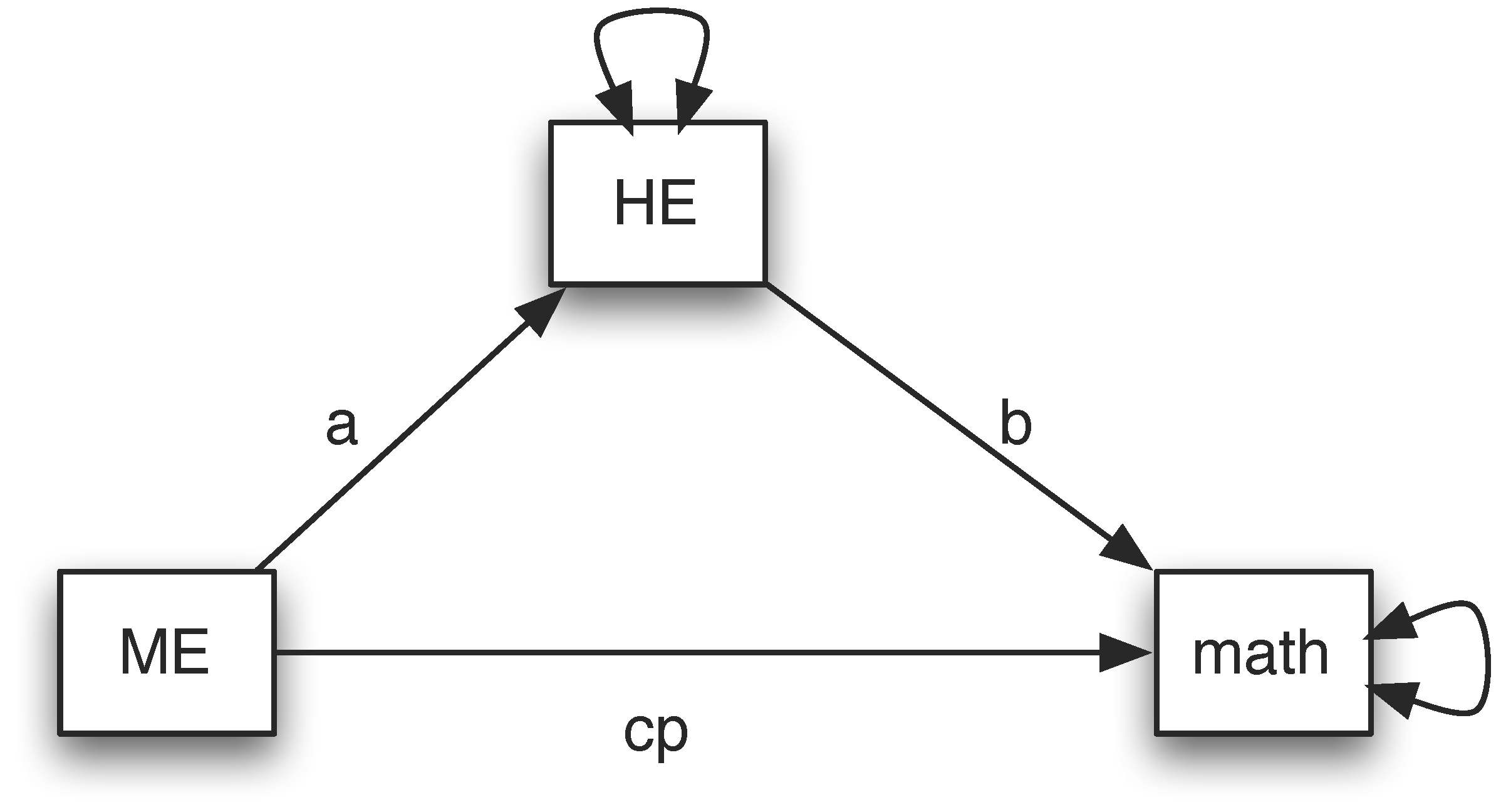
To estimate the paths in the model, we use the R package lavaan. To specify the mediation model, we follow the rules below. First, a model is put into a pair of quotation marks. Second, to specify the regression relationship, we use a symbol ~. The variable on the left is the outcome and the ones on the right are predictors or covariates. Third, parameter names can be used for paths in model specification such as a, b and cp. Fourth, we can define new parameters using the notation :=. On the left is the name of the new parameter and on the right is the formula to define the new parameter such as a*b that defines the mediation effect and a*b + cp that defines the total effect.
To estimate the model, the sem() function from lavaan can be used. To view the results, the summary() function is used. For example, for the mediation example, the output is given below. From the output, we can see
> library(lavaan)
This is lavaan 0.5-23.1097
lavaan is BETA software! Please report any bugs.
> usedata('nlsy')
>
> mediation<-'
+ math ~ b*HE + cp*ME
+ HE ~ a*ME
+ ab := a*b
+ total := a*b + cp
+ '
>
> mediation.res<-sem(mediation, data=nlsy)
> summary(mediation.res)
lavaan (0.5-23.1097) converged normally after  21 iterations

  Number of observations                           371

  Estimator                                         ML
  Minimum Function Test Statistic                0.000
  Degrees of freedom                                 0
  Minimum Function Value               0.0000000000000

Parameter Estimates:

  Information                                 Expected
  Standard Errors                             Standard

Regressions:
                   Estimate  Std.Err  z-value  P(>|z|)
  math ~
    HE         (b)    0.465    0.143    3.252    0.001
    ME        (cp)    0.463    0.120    3.869    0.000
  HE ~
    ME         (a)    0.139    0.043    3.249    0.001

Variances:
                   Estimate  Std.Err  z-value  P(>|z|)
   .math             20.621    1.514   13.620    0.000
   .HE                2.724    0.200   13.620    0.000

Defined Parameters:
                   Estimate  Std.Err  z-value  P(>|z|)
    ab                0.065    0.028    2.298    0.022
    total             0.528    0.120    4.410    0.000

>
- An individual path can be tested. For example, the coefficient from ME to HE is 0.139, which is significant based on the z-test.
- The residual variance parameters are also automatically estimated.
- The mediation effect is estimated and tested using the defined parameter. For example, the mediation effect here is 0.065 with the standard error 0.028. It is significant based on a z-test (Sobel test). Note that the result is the same as the mediation analysis before.
Example 2. Testing a theory of no direct effect
Assume we hypothesize that there is no direct effect from ME to math. To test the hypothesis, we can fit a model illustrated below.
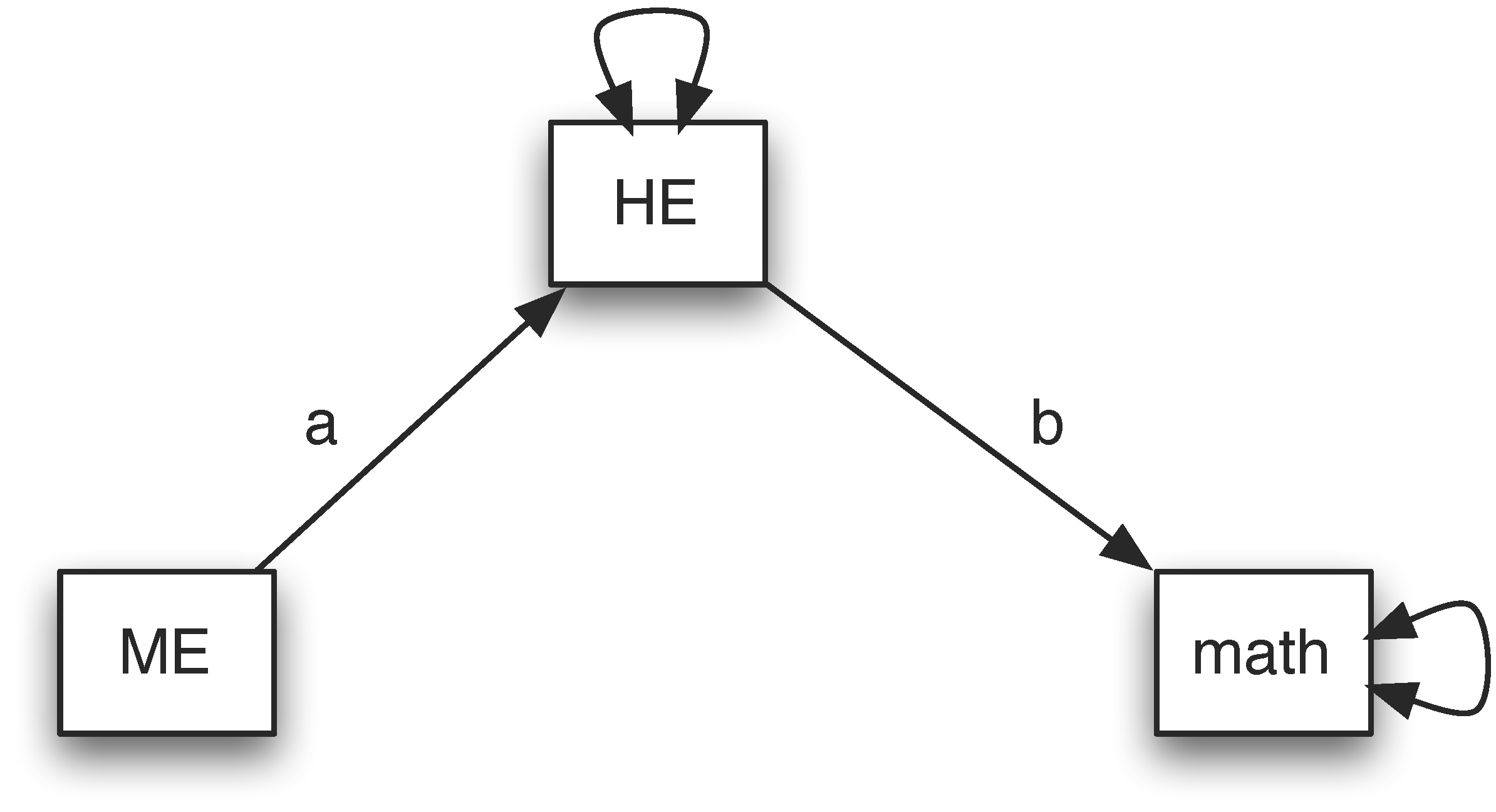
The input and output of the analysis are given below. To evaluate the hypothesis, we can check the model fit. The null hypothesis is “\(H_{0}\): The model fits the data well or the model is supported”. The alternative hypothesis is “\(H_{1}\): The model does not fit the data or the model is rejected”. The model with the direct effect fits the data perfectly. Therefore, if the current model also fits the data well, we fail to reject the null hypothesis. Otherwise, we reject it. The test of the model can be conducted based on a chi-squared test. From the output, the Chi-square is 14.676 with 1 degree of freedom. The p-value is about 0. Therefore, the null hypothesis is rejected. This indicates that the model without direct effect is not a good model.
> library(lavaan)
This is lavaan 0.5-23.1097
lavaan is BETA software! Please report any bugs.
> usedata('nlsy')
>
> model2<-'
+ math ~ b*HE
+ HE ~ a*ME
+ '
>
> model2.res<-sem(model2, data=nlsy)
> summary(model2.res)
lavaan (0.5-23.1097) converged normally after  17 iterations

  Number of observations                           371

  Estimator                                         ML
  Minimum Function Test Statistic               14.676
  Degrees of freedom                                 1
  P-value (Chi-square)                           0.000

Parameter Estimates:

  Information                                 Expected
  Standard Errors                             Standard

Regressions:
                   Estimate  Std.Err  z-value  P(>|z|)
  math ~
    HE         (b)    0.556    0.144    3.873    0.000
  HE ~
    ME         (a)    0.139    0.043    3.249    0.001

Variances:
                   Estimate  Std.Err  z-value  P(>|z|)
   .math             21.453    1.575   13.620    0.000
   .HE                2.724    0.200   13.620    0.000

>
Example 3: A more complex path model
Path analysis can be used to test more complex theories. In this example, we look at how age and education influence EPT using the ACTIVE data. Both age and education may influence EPT directly or through memory and reasoning ability. Therefore, we can fit a model shown below.
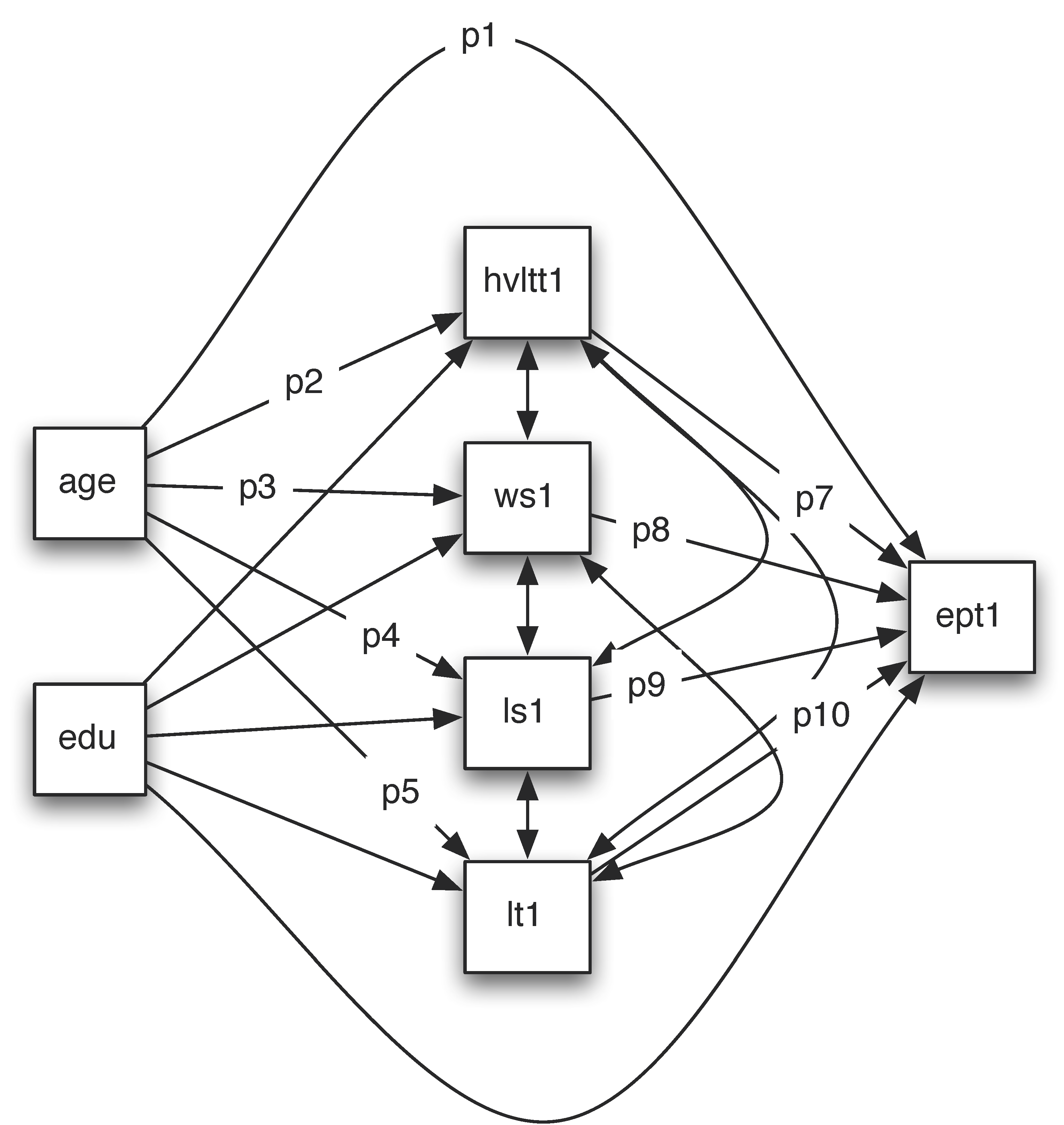
Suppose we want to test the total effect of age on EPT and its indirect effect. The direct effect is the path from age to ept1 directly, denoted by p1. One indirect path goes through hvltt1, that is p2*p7. The second indirect effect through ws1 is p3*p8. The third indirect effect through ls1 is p4*p9. The last indirect effect through lt1 is p5*p10. The total indirect effect is p2*p7+p3*p8+p4*p9+p5*p10. The total effect is the sum of them p1+p2*p7+p3*p8+p4*p9+p5*p10.
The output from such a model is given below. From it, we can see that the indirect effect ind1=p2*p7 is significant. The total indirect (indirect) from age to EPT is also significant. Finally, the total effect (total) from age to EPT is significant.
> library(lavaan)
This is lavaan 0.5-23.1097
lavaan is BETA software! Please report any bugs.
> usedata('active.full')
>
> active.model<-'
+ hvltt1 ~ p1*age + edu
+ ws1 ~ p2*age + edu
+ ls1 ~ p3*age + edu
+ lt1 ~ p4*age + edu
+ ept1 ~ p5*age + p6*edu + p7*hvltt1 + p8*ws1 + p9*ls1 + p10*lt1
+ ws1~~ls1
+ ws1~~lt1
+ ls1~~lt1
+ hvltt1~~ls1
+ hvltt1~~ws1
+ hvltt1~~lt1
+ ind1 := p1*p7
+ total := p5 + p1*p7 + p2*p8 + p3*p9 + p4*p10
+ indirect := p1*p7 + p2*p8 + p3*p9 + p4*p10
+ '
>
> active.res<-sem(active.model, data=active.full)
> summary(active.res)
lavaan (0.5-23.1097) converged normally after  79 iterations

  Number of observations                          1114

  Estimator                                         ML
  Minimum Function Test Statistic                0.000
  Degrees of freedom                                 0

Parameter Estimates:

  Information                                 Expected
  Standard Errors                             Standard

Regressions:
                   Estimate  Std.Err  z-value  P(>|z|)
  hvltt1 ~
    age       (p1)   -0.161    0.027   -6.074    0.000
    edu               0.429    0.052    8.177    0.000
  ws1 ~
    age       (p2)   -0.226    0.026   -8.737    0.000
    edu               0.704    0.051   13.772    0.000
  ls1 ~
    age       (p3)   -0.276    0.029   -9.658    0.000
    edu               0.877    0.057   15.486    0.000
  lt1 ~
    age       (p4)   -0.085    0.015   -5.894    0.000
    edu               0.394    0.029   13.723    0.000
  ept1 ~
    age       (p5)    0.014    0.021    0.644    0.519
    edu       (p6)    0.448    0.045    9.913    0.000
    hvltt1    (p7)    0.202    0.025    8.045    0.000
    ws1       (p8)    0.196    0.038    5.179    0.000
    ls1       (p9)    0.246    0.035    7.090    0.000
    lt1      (p10)    0.151    0.051    2.953    0.003

Covariances:
                   Estimate  Std.Err  z-value  P(>|z|)
 .ws1 ~~
   .ls1              16.606    0.819   20.287    0.000
   .lt1               5.714    0.371   15.390    0.000
 .ls1 ~~
   .lt1               6.573    0.415   15.852    0.000
 .hvltt1 ~~
   .ls1               8.444    0.713   11.838    0.000
   .ws1               7.572    0.643   11.769    0.000
   .lt1               2.856    0.349    8.191    0.000

Variances:
                   Estimate  Std.Err  z-value  P(>|z|)
   .hvltt1           20.618    0.874   23.601    0.000
   .ws1              19.588    0.830   23.601    0.000
   .ls1              24.030    1.018   23.601    0.000
   .lt1               6.174    0.262   23.601    0.000
   .ept1             12.177    0.516   23.601    0.000

Defined Parameters:
                   Estimate  Std.Err  z-value  P(>|z|)
    ind1             -0.033    0.007   -4.847    0.000
    total            -0.144    0.026   -5.594    0.000
    indirect         -0.158    0.017   -9.340    0.000

>
To cite the book, use:
Zhang, Z. & Wang, L. (2017-2026). Advanced statistics using R. Granger, IN: ISDSA Press. https://doi.org/10.35566/advstats. ISBN: 978-1-946728-01-2.
To take the full advantage of the book such as running analysis within your web browser, please subscribe.