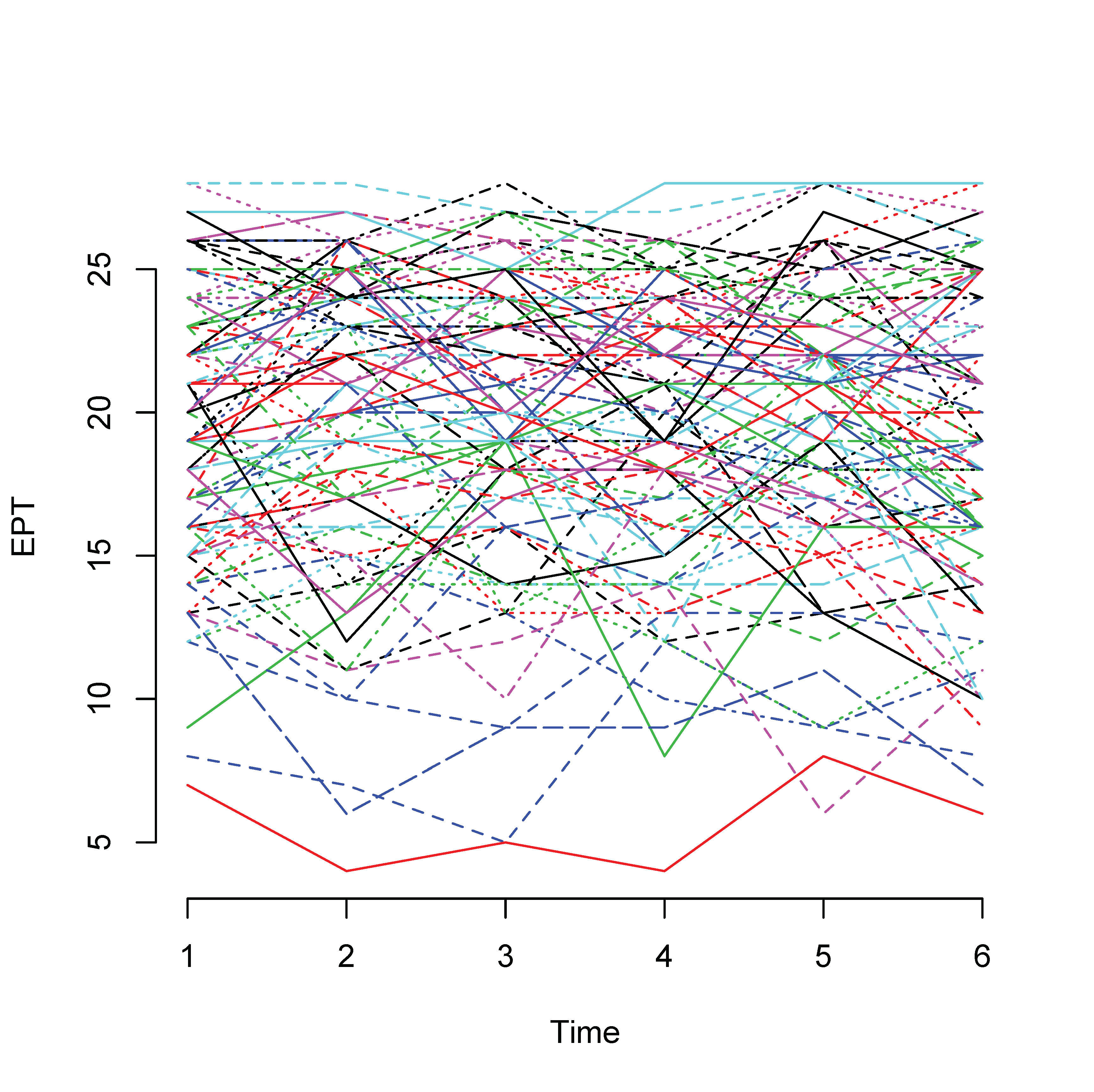
Longitudinal data can be viewed as a special case of the multilevel data where time is nested within individual participants. All longitudinal data share at least three features: (1) the same entities are repeatedly observed over time; (2) the same measurements (including parallel tests) are used; and (3) the timing for each measurement is known (Baltes & Nesselroade, 1979). To study phenomena in their time-related patterns of constancy and change is a primary reason for collecting longitudinal data. Figure 1 show the plot of 50 participants from the ACTIVE study on the variable EPT for 6 times. Clearly, each line represents a participant. From it, we can see how an individual changes over time.
1. A plot of longitudinal data
Growth curve model
Growth curve models (GCM; e.g., McArdle \& Nesselroade, 2003; Meredith & Tisak, 1990) exemplify a widely used technique with a direct match to the objectives of longitudinal research described by Baltes and Nesselroade (1979) to analyze explicitly intra-individual change and inter-individual differences in change. In the past decades, growth curve models have evolved from fitting a single curve for only one individual to fitting multilevel or mixed-effects models and from linear to nonlinear models (e.g., McArdle, 2001; McArdle & Nesselroade, 2003; Meredith & Tisak, 1990; Tucker, 1958; Wishart, 1938).
A typical linear growth curve model can be written as
where $y_{it}$ is data for participant $i$ at time $t$. For each individual $i$, a linear regression model can be fitted with its own intercept $\beta_{0i}$ and slope $\beta_{1i}$. On average, there is an intercept $\gamma_{0}$ and slope $\gamma_{1}$ for all individuals. The variation of $\beta_{0i}$ and $\beta_{1i}$ represents individual differences.
Individual difference can be further explained by other factors, for example, education level and age. Then the model is
For demonstration, we investigate the growth of word set test (ws in the ACTIVE data set). In the current data set, we have the data in wide format, in which the 6 measures of ws are 6 variables. To use the R package, long format data are needed. For the long-format data, we need to stack the data from all waves into a long variable. The R code below reformats the data and plot them.
Unconditional model (model without second level predictors)
Fitting the model is actually straightforward using the lmer() function. The input and output are given below. Based on the output, the fixed effects for time (.214, t-value=11.59) is significant, therefore, there is a linear growth trend. The average intercept is 11.93 and is also significant.
> library(lme4)
Loading required package: Matrix
> library(lmerTest)

Attaching package: 'lmerTest'

The following object is masked from 'package:lme4':

    lmer

The following object is masked from 'package:stats':

    step

> usedata('active.full')
> attach(active.full)
> longdata<-data.frame(ws=c(ws1,ws2,ws3,ws4,ws5,ws6),
+                      parti=factor(rep(paste('p', 1:1114, sep=''), 6)),
+                      time=rep(1:6, each=1114),
+                      edu=rep(edu, 6))
>
> m1<-lmer(ws~time+(1+time|parti), data=longdata)
> summary(m1)
Linear mixed model fit by REML t-tests use Satterthwaite approximations to
  degrees of freedom [lmerMod]
Formula: ws ~ time + (1 + time | parti)
   Data: longdata

REML criterion at convergence: 34088.3

Scaled residuals:
    Min      1Q  Median      3Q     Max
-4.3918 -0.5446 -0.0163  0.5643  4.4923

Random effects:
 Groups   Name        Variance Std.Dev. Corr
 parti    (Intercept) 21.11487 4.5951
          time         0.07364 0.2714   0.15
 Residual              5.36089 2.3154
Number of obs: 6684, groups:  parti, 1114

Fixed effects:
             Estimate Std. Error        df t value Pr(>|t|)
(Intercept) 1.193e+01  1.521e-01 1.113e+03   78.42   <2e-16 ***
time        2.140e-01  1.847e-02 1.113e+03   11.59   <2e-16 ***
---
Signif. codes:  0 '***' 0.001 '**' 0.01 '*' 0.05 '.' 0.1 ' ' 1

Correlation of Fixed Effects:
     (Intr)
time -0.285
> anova(m1)
Analysis of Variance Table of type III  with  Satterthwaite
approximation for degrees of freedom
     Sum Sq Mean Sq NumDF DenDF F.value    Pr(>F)
time 720.14  720.14     1  1113  134.33 < 2.2e-16 ***
---
Signif. codes:  0 '***' 0.001 '**' 0.01 '*' 0.05 '.' 0.1 ' ' 1
>
It is useful to test whether random-effects parameters such as the variances of intercept and slope are significance or not to evaluate individual differences. This can be done by comparing the current model with a model without random intercept or slope.
For example, to test the individual differences in slope for time. The random effects for time is .07. Based on ANOVA analysis, it is significant with p-value about 0. Therefore, there is significant individual difference in the growth rate (slope). This indicates that everyone has a different change rate. Note that in m1.alt, the random effect for time was not used.
> library(lme4)
Loading required package: Matrix
> library(lmerTest)

Attaching package: 'lmerTest'

The following object is masked from 'package:lme4':

    lmer

The following object is masked from 'package:stats':

    step

> usedata('active.full')
> attach(active.full)
> longdata<-data.frame(ws=c(ws1,ws2,ws3,ws4,ws5,ws6),
+                      parti=factor(rep(paste('p', 1:1114, sep=''), 6)),
+                      time=rep(1:6, each=1114),
+                      edu=rep(edu, 6))
>
> m1<-lmer(ws~time+(1+time|parti), data=longdata)
>
> m1.alt1<-lmer(ws~time+(1|parti), data=longdata)
> summary(m1.alt1)
Linear mixed model fit by REML t-tests use Satterthwaite approximations to
  degrees of freedom [lmerMod]
Formula: ws ~ time + (1 | parti)
   Data: longdata

REML criterion at convergence: 34133.4

Scaled residuals:
    Min      1Q  Median      3Q     Max
-4.7097 -0.5452  0.0030  0.5784  4.5111

Random effects:
 Groups   Name        Variance Std.Dev.
 parti    (Intercept) 23.243   4.821
 Residual              5.618   2.370
Number of obs: 6684, groups:  parti, 1114

Fixed effects:
             Estimate Std. Error        df t value Pr(>|t|)
(Intercept) 1.193e+01  1.589e-01 1.497e+03   75.07   <2e-16 ***
time        2.140e-01  1.698e-02 5.569e+03   12.61   <2e-16 ***
---
Signif. codes:  0 '***' 0.001 '**' 0.01 '*' 0.05 '.' 0.1 ' ' 1

Correlation of Fixed Effects:
     (Intr)
time -0.374
>
> anova(m1, m1.alt1)
refitting model(s) with ML (instead of REML)
Data: longdata
Models:
..1: ws ~ time + (1 | parti)
object: ws ~ time + (1 + time | parti)
       Df   AIC   BIC logLik deviance Chisq Chi Df Pr(>Chisq)
..1     4 34133 34160 -17063    34125
object  6 34092 34133 -17040    34080    45      2  1.692e-10 ***
---
Signif. codes:  0 '***' 0.001 '**' 0.01 '*' 0.05 '.' 0.1 ' ' 1
>
To test the individual differences in intercept. The random effects for intercept is 21.11. Based on ANOVA analysis below, it is significant. Therefore, there is individual difference or individuals have different intercepts.
> library(lme4)
Loading required package: Matrix
> library(lmerTest)

Attaching package: 'lmerTest'

The following object is masked from 'package:lme4':

    lmer

The following object is masked from 'package:stats':

    step

> usedata('active.full')
> attach(active.full)
> longdata<-data.frame(ws=c(ws1,ws2,ws3,ws4,ws5,ws6),
+                      parti=factor(rep(paste('p', 1:1114, sep=''), 6)),
+                      time=rep(1:6, each=1114),
+                      edu=rep(edu, 6))
>
> m1<-lmer(ws~time+(1+time|parti), data=longdata)
>
> m1.alt2<-lmer(ws~time+(time-1|parti), data=longdata)
> summary(m1.alt2)
Linear mixed model fit by REML t-tests use Satterthwaite approximations to
  degrees of freedom [lmerMod]
Formula: ws ~ time + (time - 1 | parti)
   Data: longdata

REML criterion at convergence: 37278

Scaled residuals:
    Min      1Q  Median      3Q     Max
-3.0574 -0.5435 -0.0079  0.5204  4.5639

Random effects:
 Groups   Name Variance Std.Dev.
 parti    time  1.228   1.108
 Residual      10.230   3.198
Number of obs: 6684, groups:  parti, 1114

Fixed effects:
             Estimate Std. Error        df t value Pr(>|t|)
(Intercept) 1.193e+01  8.921e-02 5.569e+03 133.680  < 2e-16 ***
time        2.140e-01  4.034e-02 1.986e+03   5.306 1.24e-07 ***
---
Signif. codes:  0 '***' 0.001 '**' 0.01 '*' 0.05 '.' 0.1 ' ' 1

Correlation of Fixed Effects:
     (Intr)
time -0.510
>
> anova(m1, m1.alt2)
refitting model(s) with ML (instead of REML)
Data: longdata
Models:
..1: ws ~ time + (time - 1 | parti)
object: ws ~ time + (1 + time | parti)
       Df   AIC   BIC logLik deviance Chisq Chi Df Pr(>Chisq)
..1     4 37278 37305 -18635    37270
object  6 34092 34133 -17040    34080  3190      2  < 2.2e-16 ***
---
Signif. codes:  0 '***' 0.001 '**' 0.01 '*' 0.05 '.' 0.1 ' ' 1
>
Conditional model (model with second level predictors)
Using the same set of data, we now investigate whether education is a predictor of random intercept and slope. Given there is individual differences in intercept and slope, we want to explain why. So, we use Edu as a explanatory variable. From the output, we can see that the parameter \(\gamma_{1} = .78\) is significant. Higher education relates to bigger intercept. In addition, the parameter $\gamma_{3} = -.022$ is significant. Higher education relates to lower growth rate of ws.
> library(lme4)
Loading required package: Matrix
> library(lmerTest)

Attaching package: 'lmerTest'

The following object is masked from 'package:lme4':

    lmer

The following object is masked from 'package:stats':

    step

> usedata('active.full')
> attach(active.full)
> longdata<-data.frame(ws=c(ws1,ws2,ws3,ws4,ws5,ws6),
+                      parti=factor(rep(paste('p', 1:1114, sep=''), 6)),
+                      time=rep(1:6, each=1114),
+                      edu=rep(edu, 6))
>
> m2<-lmer(ws~time+edu+time*edu+(1+time|parti), data=longdata)
> summary(m2)
Linear mixed model fit by REML t-tests use Satterthwaite approximations to
  degrees of freedom [lmerMod]
Formula: ws ~ time + edu + time * edu + (1 + time | parti)
   Data: longdata

REML criterion at convergence: 33907.6

Scaled residuals:
    Min      1Q  Median      3Q     Max
-4.3732 -0.5494 -0.0160  0.5700  4.3767

Random effects:
 Groups   Name        Variance Std.Dev. Corr
 parti    (Intercept) 17.04402 4.1284
          time         0.07046 0.2654   0.27
 Residual              5.36089 2.3154
Number of obs: 6684, groups:  parti, 1114

Fixed effects:
              Estimate Std. Error         df t value Pr(>|t|)
(Intercept)  1.240e+00  7.506e-01  1.112e+03   1.652   0.0987 .
time         5.276e-01  9.894e-02  1.112e+03   5.332 1.17e-07 ***
edu          7.779e-01  5.369e-02  1.112e+03  14.488  < 2e-16 ***
time:edu    -2.282e-02  7.077e-03  1.112e+03  -3.225   0.0013 **
---
Signif. codes:  0 '***' 0.001 '**' 0.01 '*' 0.05 '.' 0.1 ' ' 1

Correlation of Fixed Effects:
         (Intr) time   edu
time     -0.270
edu      -0.983  0.265
time:edu  0.265 -0.983 -0.270
> anova(m2)
Analysis of Variance Table of type III  with  Satterthwaite
approximation for degrees of freedom
          Sum Sq Mean Sq NumDF DenDF F.value    Pr(>F)
time      152.43  152.43     1  1112  28.434 1.174e-07 ***
edu      1125.20 1125.20     1  1112 209.890 < 2.2e-16 ***
time:edu   55.76   55.76     1  1112  10.400  0.001297 **
---
Signif. codes:  0 '***' 0.001 '**' 0.01 '*' 0.05 '.' 0.1 ' ' 1
>
GCM as a SEM
In addition to estimating a GCM as a multilevel or mixed-effects model, we can also estimate it as a SEM. To illustrate this, we consider a linear growth curve model. If a group of participants all have linear change trend, for each individual, we can fit a regression model such as \[ y_{it}=\beta_{i0}+\beta_{i1}t+e_{it} \] where $\beta_{i0}$ and $\beta_{i1}$ are intercept and slope, respectively. Note that here we let $time_{it} = t$. If each individual has different time of data collection, it can still be done in the SEM framework but would be more complex. By writing the time out, we would have
\[ \left(\begin{array}{c} y_{i1}\\ y_{i2}\\ \vdots\\ y_{iT} \end{array}\right)=\left(\begin{array}{cc} 1 & 1\\ 1 & 2\\ 1 & \vdots\\ 1 & T \end{array}\right)\left(\begin{array}{c} \beta_{i0}\\ \beta_{i1} \end{array}\right)+\left(\begin{array}{c} e_{i1}\\ e_{i2}\\ \vdots\\ e_{iT} \end{array}\right) \]
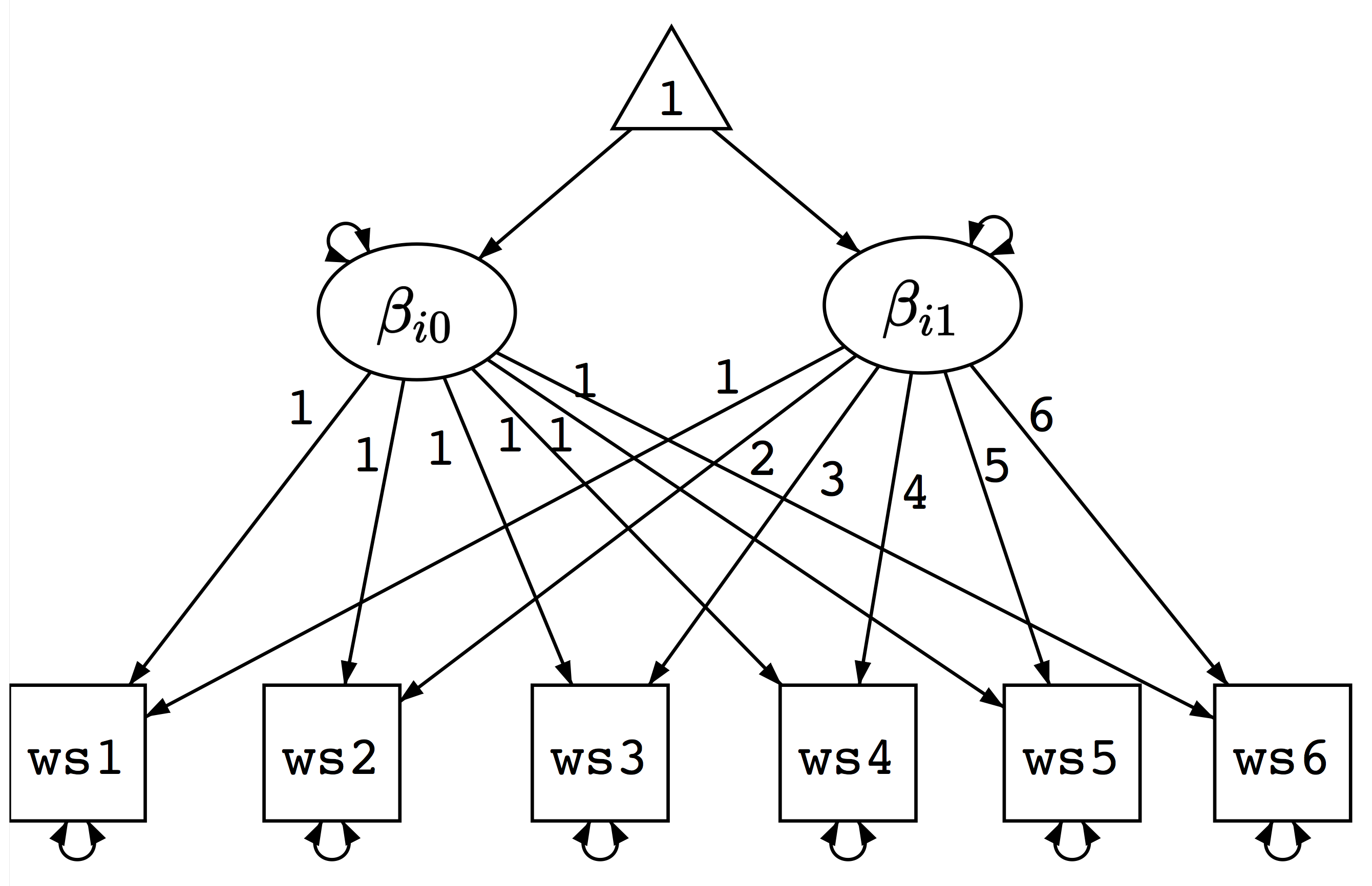
Note that the above equation resembles a factor model with two factors - $b_{0}$ and $b_{1}$ and a factor loading matrix with known factor loading matrix. The individual intercept and slope can be viewed as factor scores to be estimated. Furthermore, we are interested in model with mean structure because the means of $\beta_{0}$ and $\beta_{1}$ have their meaning as average intercept and slope (rate of change). The variances of the factors can be estimated - they indicate the variations of intercept and slope. Using path diagram, the model is shown in the figure below.
2. Path diagram for a growth curve model
With the model, we can estimate it using the sem() function in the lavaan package. Because of the frequent use of growth curve model, the package also provides a function growth() to ease such analysis. Unlike the lme4 package, in using SEM, the wide format of data is directly used. The R input and output for the unconditional model is given below.
Note that the gcm() function works similarly as sem() function. Using this method, each parameter in the model can be directly tested using a z-test. In addition, we can use the fit statistics for SEM to test the fit of the growth curve model. Particularly for the current analysis, the linear growth curve model does not seem to fit the data well.
> library(lavaan)
This is lavaan 0.5-23.1097
lavaan is BETA software! Please report any bugs.
> usedata('active.full')
>
> gcm <- '
+ beta0 =~ 1*ws1 + 1*ws2 + 1*ws3 + 1*ws4 + 1*ws5 + 1*ws6
+ beta1 =~ 1*ws1 + 2*ws2 + 3*ws3 + 4*ws4 + 5*ws5 + 6*ws6
+ '
>
> gcm.res <- growth(gcm, data=active.full)
Warning message:
In lav_object_post_check(object) :
  lavaan WARNING: some estimated lv variances are negative
> summary(gcm.res, fit=TRUE)
lavaan (0.5-23.1097) converged normally after  53 iterations

  Number of observations                          1114

  Estimator                                         ML
  Minimum Function Test Statistic              691.253
  Degrees of freedom                                16
  P-value (Chi-square)                           0.000

Model test baseline model:

  Minimum Function Test Statistic             8065.569
  Degrees of freedom                                15
  P-value                                        0.000

User model versus baseline model:

  Comparative Fit Index (CFI)                    0.916
  Tucker-Lewis Index (TLI)                       0.921

Loglikelihood and Information Criteria:

  Loglikelihood user model (H0)             -16958.575
  Loglikelihood unrestricted model (H1)     -16612.949

  Number of free parameters                         11
  Akaike (AIC)                               33939.151
  Bayesian (BIC)                             33994.324
  Sample-size adjusted Bayesian (BIC)        33959.385

Root Mean Square Error of Approximation:

  RMSEA                                          0.195
  90 Percent Confidence Interval          0.182  0.207
  P-value RMSEA <= 0.05                          0.000

Standardized Root Mean Square Residual:

  SRMR                                           0.095

Parameter Estimates:

  Information                                 Expected
  Standard Errors                             Standard

Latent Variables:
                   Estimate  Std.Err  z-value  P(>|z|)
  beta0 =~
    ws1               1.000
    ws2               1.000
    ws3               1.000
    ws4               1.000
    ws5               1.000
    ws6               1.000
  beta1 =~
    ws1               1.000
    ws2               2.000
    ws3               3.000
    ws4               4.000
    ws5               5.000
    ws6               6.000

Covariances:
                   Estimate  Std.Err  z-value  P(>|z|)
  beta0 ~~
    beta1             0.406    0.106    3.817    0.000

Intercepts:
                   Estimate  Std.Err  z-value  P(>|z|)
   .ws1               0.000
   .ws2               0.000
   .ws3               0.000
   .ws4               0.000
   .ws5               0.000
   .ws6               0.000
    beta0            12.263    0.155   79.217    0.000
    beta1             0.161    0.018    8.770    0.000

Variances:
                   Estimate  Std.Err  z-value  P(>|z|)
   .ws1               8.999    0.443   20.293    0.000
   .ws2               5.614    0.284   19.751    0.000
   .ws3               3.867    0.209   18.539    0.000
   .ws4               4.091    0.219   18.639    0.000
   .ws5               4.712    0.249   18.915    0.000
   .ws6               6.420    0.343   18.723    0.000
    beta0            20.854    1.143   18.246    0.000
    beta1            -0.004    0.019   -0.186    0.853

>
Fitting a conditional model is similar but one would need to use the predictor for the factors.
> library(lavaan)
This is lavaan 0.5-23.1097
lavaan is BETA software! Please report any bugs.
> usedata('active.full')
>
> gcm2 <- '
+ beta0 =~ 1*ws1 + 1*ws2 + 1*ws3 + 1*ws4 + 1*ws5 + 1*ws6
+ beta1 =~ 1*ws1 + 2*ws2 + 3*ws3 + 4*ws4 + 5*ws5 + 6*ws6
+ beta0 ~ edu
+ beta1 ~ edu
+ '
>
> gcm2.res <- growth(gcm2, data=active.full)
Warning message:
In lav_object_post_check(object) :
  lavaan WARNING: some estimated lv variances are negative
> summary(gcm2.res, fit=TRUE)
lavaan (0.5-23.1097) converged normally after  54 iterations

  Number of observations                          1114

  Estimator                                         ML
  Minimum Function Test Statistic              697.223
  Degrees of freedom                                20
  P-value (Chi-square)                           0.000

Model test baseline model:

  Minimum Function Test Statistic             8259.498
  Degrees of freedom                                21
  P-value                                        0.000

User model versus baseline model:

  Comparative Fit Index (CFI)                    0.918
  Tucker-Lewis Index (TLI)                       0.914

Loglikelihood and Information Criteria:

  Loglikelihood user model (H0)             -19509.237
  Loglikelihood unrestricted model (H1)     -19160.626

  Number of free parameters                         13
  Akaike (AIC)                               39044.475
  Bayesian (BIC)                             39109.679
  Sample-size adjusted Bayesian (BIC)        39068.388

Root Mean Square Error of Approximation:

  RMSEA                                          0.174
  90 Percent Confidence Interval          0.163  0.186
  P-value RMSEA <= 0.05                          0.000

Standardized Root Mean Square Residual:

  SRMR                                           0.083

Parameter Estimates:

  Information                                 Expected
  Standard Errors                             Standard

Latent Variables:
                   Estimate  Std.Err  z-value  P(>|z|)
  beta0 =~
    ws1               1.000
    ws2               1.000
    ws3               1.000
    ws4               1.000
    ws5               1.000
    ws6               1.000
  beta1 =~
    ws1               1.000
    ws2               2.000
    ws3               3.000
    ws4               4.000
    ws5               5.000
    ws6               6.000

Regressions:
                   Estimate  Std.Err  z-value  P(>|z|)
  beta0 ~
    edu               0.782    0.055   14.290    0.000
  beta1 ~
    edu              -0.023    0.007   -3.348    0.001

Covariances:
                   Estimate  Std.Err  z-value  P(>|z|)
 .beta0 ~~
   .beta1             0.531    0.098    5.416    0.000

Intercepts:
                   Estimate  Std.Err  z-value  P(>|z|)
   .ws1               0.000
   .ws2               0.000
   .ws3               0.000
   .ws4               0.000
   .ws5               0.000
   .ws6               0.000
   .beta0             1.510    0.765    1.974    0.048
   .beta1             0.486    0.098    4.959    0.000

Variances:
                   Estimate  Std.Err  z-value  P(>|z|)
   .ws1               8.860    0.434   20.406    0.000
   .ws2               5.641    0.283   19.939    0.000
   .ws3               3.903    0.209   18.686    0.000
   .ws4               4.090    0.219   18.637    0.000
   .ws5               4.717    0.249   18.921    0.000
   .ws6               6.428    0.342   18.772    0.000
   .beta0            16.695    0.968   17.246    0.000
   .beta1            -0.006    0.019   -0.340    0.734

>
To cite the book, use:
Zhang, Z. & Wang, L. (2017-2026). Advanced statistics using R. Granger, IN: ISDSA Press. https://doi.org/10.35566/advstats. ISBN: 978-1-946728-01-2. To take the full advantage of the book such as running analysis within your web browser, please subscribe.