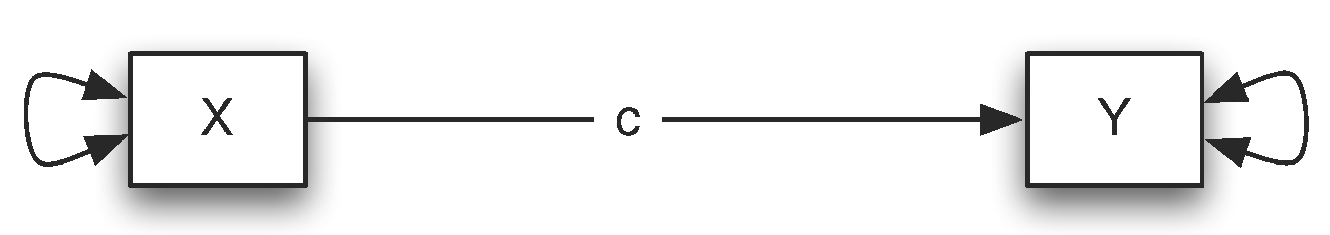
To explain what is a moderator, we start with a bivariate relationship between an input variable X and an outcome variable $Y$. For example, $X$ could be the number of training sessions (training intensity) and $Y$ could be math test score. We can hypothesize that there is a relationship between them such that the number of training sessions predicts math test performance. Using a diagram, we can portray the relationship below.
The above path diagram can be expressed using a regression model as
\[ Y=\beta_{0}+\beta_{1}*X+\epsilon \]
where $\beta_{0}$ is the intercept and $\beta_{1}$ is the slope.
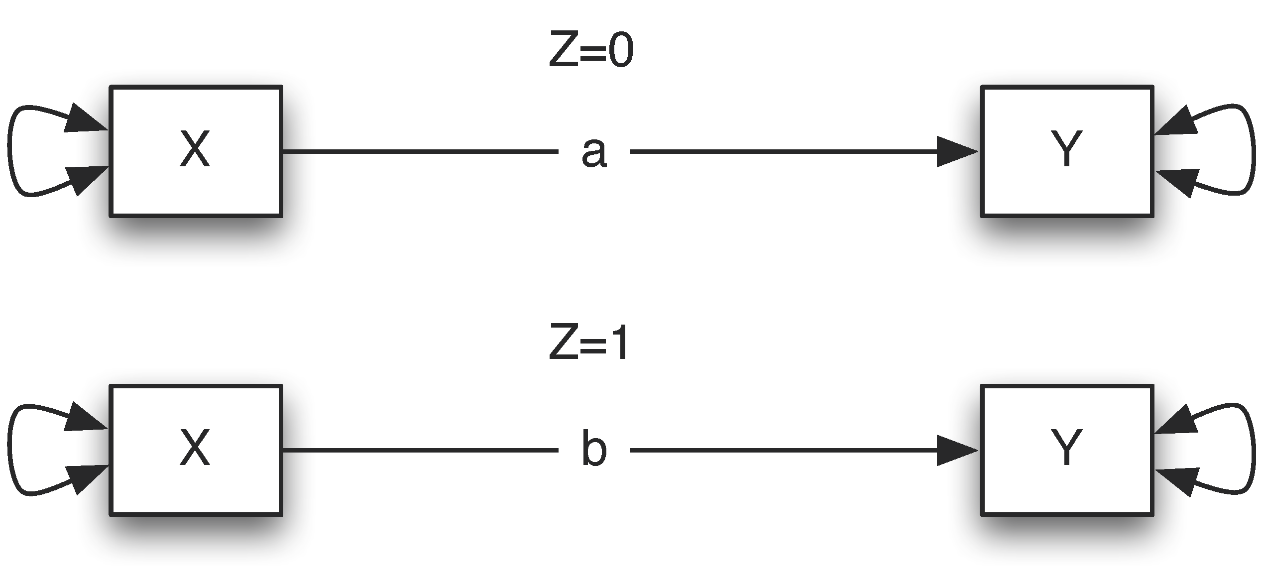
A moderator variable Z is a variable that alters the strength of the relationship between $X$ and $Y$. In other words, the effect of $X$ on $Y$ depends on the levels of the moderator $Z$. For instance, if male students ($Z=0$) benefit more (or less) from training than female students ($Z=1$), then gender can be considered as a moderator. Using the diagram, if the coefficient $a$ is different $b$, there is a moderation effect.
To summarize, a moderator $Z$ is a variable that alters the direction and/or strength of the relation between a predictor $X$ and an outcome $Y$.
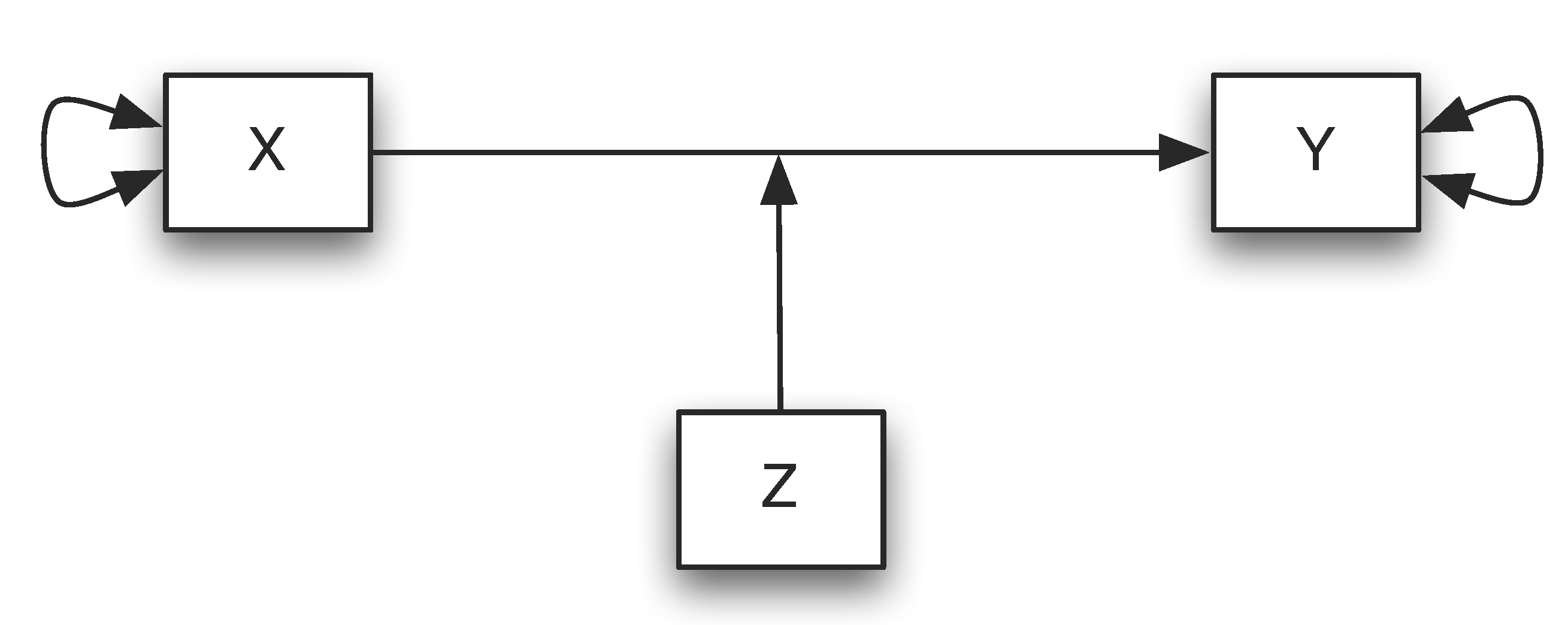
Questions involving moderators address “when” or “for whom” a variable most strongly predicts or causes an outcome variable. Using a path diagram, we can express the moderation effect as:
How to conduct moderation analysis?
Moderation analysis can be conducted by adding one or multiple interaction terms in a regression analysis. For example, if $Z$ is a moderator for the relation between $X$ and $Y$, we can fit a regression model
Thus, if \(\beta_{3}\) is not equal to 0, the relationship between $X$ and $Y$ depends on the value of $Z$, which indicates a moderation effect. In fact, from the regression model, we can get:
If $z=0$, the effect of $X$ on Y is $\beta_{1}+\beta_{3}*0=\beta_{1}$.
If $z=2$, the effect of $X$ on Y is $\beta_{1}+\beta_{3}*2$.
If $z=4$, the effect of $X$ on Y is $\beta_{1}+\beta_{3}*4$.
If $Z$ is a dichotomous/binary variable, for example, gender, the above equation can be written as
Thus, if $\beta_{3}$ is not equal to 0, the relationship between X and Y depends on the value of $Z$, which indicates a moderation effect. When $z=0,$ the effect of $X$ on Y is $\beta_{1}+\beta_{3}*0=\beta_{1}$ and when $z=1$, the effect of $X$ on Y is $\beta_{1}+\beta_{3}*1$ for female students.
Steps for moderation analysis
A moderation analysis typically consists of the following steps.
Compute the interaction term XZ=X*Z.
Fit a multiple regression model with X, Z, and XZ as predictors.
Test whether the regression coefficient for XZ is significant or not.
Interpret the moderation effect.
Display the moderation effect graphically.
An example
The data set mathmod.csv includes three variables: training intensity, gender, and math test score. Using the example, we investigate whether the effect of training intensity on math test performance depends on gender. Therefore, we evaluate whether gender is a moderator.
The R code for the analysis is given below.
> usedata('mathmod'); attach(mathmod);
>
> # Computer the interaction term
> xz<-training*gender
> summary(lm(math~training+gender+xz))

Call:
lm(formula = math ~ training + gender + xz)

Residuals:
    Min      1Q  Median      3Q     Max
-2.6837 -0.5892 -0.1057  0.7811  2.2350

Coefficients:
            Estimate Std. Error t value Pr(>|t|)
(Intercept)  4.98999    0.27499  18.146  < 2e-16 ***
training    -0.33943    0.05387  -6.301 8.70e-09 ***
gender      -2.75688    0.37912  -7.272 9.14e-11 ***
xz           0.50427    0.06845   7.367 5.80e-11 ***
---
Signif. codes:  0 '***' 0.001 '**' 0.01 '*' 0.05 '.' 0.1 ' ' 1

Residual standard error: 0.9532 on 97 degrees of freedom
Multiple R-squared:  0.3799,	Adjusted R-squared:  0.3607
F-statistic: 19.81 on 3 and 97 DF,  p-value: 4.256e-10

>
Since the regression coefficient (0.504) for the interaction term XZ is significant at the alpha level 0.05 with a p-value=5.8e-11, there exists a significant moderation effect. In other words, the effect of training intensity on math performance significantly depends on gender.
When Z=0 (male students), the estimated effect of training intensity on math performance is \(\hat{\beta}_{1}=-.34\). When Z=1 (female students), the estimated effect of training intensity on math performance is \(\hat{\beta}_{1}+\hat{\beta}_{3}=-.34+.50=.16\). The moderation analysis tells us that the effects of training intensity on math performance for males (-.34) and females (.16) are significantly different for this example.
Interaction plot
A moderation effect indicates the regression slopes are different for different groups. Therefore, if we plot the regression line for each group, they should interact at certain point. Such a plot is called an interaction plot. To get the plot, we first calculate the intercept and slope for each level of the moderator. For this example, we have
With the information, we can generate a plot using the R code below. Note that the option type='n' generates a figure without actually plotting the data. In the function abline(), the first value is the intercept and the second is the slope. Note that the values for each level can also be added to the plot.
The data set depress.csv includes three variables: Stress, Social support and Depression. Suppose we want to investigate whether social support is a moderator for the relation between stress and depression. That is, to study whether the effect of stress on depression depends on different levels of social support. Note that the potential moderator social support is a continuous variable.
The analysis is given below. The regression coefficient estimate of the interaction term is -.39 with t = -20.754, p <.001. Therefore, social support is a significant moderator for the relation between stress and depression. The relation between stress and depression significantly depends on different levels of social support.
> usedata('depress');
>
> # the interaction term
> depress$inter<-depress$stress*depress$support
> summary(lm(depress~stress+support+inter, data=depress))

Call:
lm(formula = depress ~ stress + support + inter, data = depress)

Residuals:
    Min      1Q  Median      3Q     Max
-3.7322 -0.9035 -0.1127  0.8542  3.6089

Coefficients:
            Estimate Std. Error t value Pr(>|t|)
(Intercept)  29.2583     0.6909  42.351   <2e-16 ***
stress        1.9956     0.1161  17.185   <2e-16 ***
support      -0.2356     0.1109  -2.125   0.0362 *
inter        -0.3902     0.0188 -20.754   <2e-16 ***
---
Signif. codes:  0 '***' 0.001 '**' 0.01 '*' 0.05 '.' 0.1 ' ' 1

Residual standard error: 1.39 on 96 degrees of freedom
Multiple R-squared:  0.9638,	Adjusted R-squared:  0.9627
F-statistic:   853 on 3 and 96 DF,  p-value: < 2.2e-16

>
Since social support is a continuous variable, there is no immediate levels to look at the relationship between stress and depression. However, we can choose several difference levels. One way is to use these three levels of a moderator: mean, one standard deviation below the mean and one standard deviation above the mean. For this example, the three values for social support are 5.37, 2.56 and 8.18. The fitted regression lines for the three values are
From it, we can clearly see that with more social support, the relationship between depression and stress becomes negative from positive. This can also be seen from the interaction plot below.
> usedata('depress');
>
> ## create an empty frame
> plot(depress$stress, depress$depress, type='n',
+      xlab='Stress', ylab='Depression')
>
> ## abline(interceptvalue, linearslopevalue)
> # for support = mean -1SD
> abline(28.65, 1)
> # for support = mean
> abline(27.97, -.09, col='blue')
> # for support = mean +1SD
> abline(27.30, -1.19, col='red')
>
> legend('topleft', c('Low', 'Medium', 'High'),
+                   lty=c(1,1,1),
+                   col=c('black','blue','red'))
>
To cite the book, use:
Zhang, Z. & Wang, L. (2017-2026). Advanced statistics using R. Granger, IN: ISDSA Press. https://doi.org/10.35566/advstats. ISBN: 978-1-946728-01-2. To take the full advantage of the book such as running analysis within your web browser, please subscribe.