Regression with Categorical Predictors
In the variable selection example, we have a predictor -- race, which has three categories: 1 = white, 2 = black, 3 = other. In the previous example, we blindly treated it as continuous by taking the numbers literally. This can cause problems. For example, when we interpret the regression slope, we say how much change in the outcome for one unit change the predictor. Although numerically it is fine to say the change from 1 to 2 is the same as the change from 2 to 3, it does not make sense at all to compare the change in the actual race categories. Therefore, although the categories are coded using numerical values, they should be treated as discrete values. This kind variables is called nominal variables. A typical example is ANOVA where the different levels of a factor should be treated as discrete values. In regression, such variables need special treatment for valid statistical inference. We show how to conduct such regression analysis through an example.
An example
In this example, we study the mid-career median salary of college graduates. The data set college.csv includes the information on salary and college backgrounds. Specifically, there are 6 variables in the data set: id, name of the college, mid-career median salary of graduates, cost of study, whether the college is public (1) or private (0), and the location of the college: 1, Southern colleges; 2, Midwestern; 3, Northeastern; and 4, Western. A subset of the data as well as some summary information are given below. In total, there are 85 colleges in the data and 50 of them are private colleges. Clearly, the variables public and location in the data set should be treated as categorical variables. Using this example, we study the factors related to median salary.
> usedata('college')
> head(college)
  id                                        name salary   cost public location
1  1 Massachusetts Institute of Technology (MIT) 119000 189300      0        3
2  2                          Harvard University 121000 189600      0        3
3  3                           Dartmouth College 123000 188400      0        3
4  4                        Princeton University 123000 188700      0        3
5  5                             Yale University 110000 194200      0        3
6  6                    University of Notre Dame 112000 181900      0        2
> attach(college)
> table(public)
public
 0  1
50 35
> table(location)
location
 1  2  3  4
20 19 25 21
>
A naive analysis
Suppose we simply treat the variables public and location and fit a multiple regression model to directly. Then, we would get the results as shown below. Then the regression model is
\[ salary = 105.48 - 11.679*public - 1.869*location. \]
Using the typical way to interpret the regression coefficients, we would say (1) when public=0 and location=0, the average salary is 105.48; (2) when public changes from 0 to 1, the salary would reduce 11.679; and (3) when location increases 1, the salary decreases 1.869. Clearly, (1) and (3) do not make sense at all even though (2) seems to be ok.
> usedata('college'); attach(college)
> salary <- salary / 1000
> summary(lm(salary ~ public + location))

Call:
lm(formula = salary ~ public + location)

Residuals:
     Min       1Q   Median       3Q      Max
-23.1028  -6.5626  -0.2319   6.1280  26.6758

Coefficients:
            Estimate Std. Error t value Pr(>|t|)
(Intercept)  105.480      2.905  36.307  < 2e-16 ***
public       -11.679      2.270  -5.145 1.79e-06 ***
location      -1.869      1.015  -1.842   0.0691 .
---
Signif. codes:  0 '***' 0.001 '**' 0.01 '*' 0.05 '.' 0.1 ' ' 1

Residual standard error: 10.27 on 82 degrees of freedom
Multiple R-squared:  0.278,	Adjusted R-squared:  0.2604
F-statistic: 15.78 on 2 and 82 DF,  p-value: 1.588e-06

>
By fitting the above regression model, we assume that each predictor has equal interval in their values. For example, for the location variable, the change from Southern to Midwestern is the same as the change from Midwestern to Northeastern. This assumption is certainly questionable for variables with distinct, non-numerical categories. The location variable here is a categorical variable, not a continuous one. The use of numerical values in the data file for categorical variables is for convenience of data input and storage and should be viewed as discrete instead of continuous values. For example, for the "public" variable, 0 should read as private and 1 should read as public. Similarly, for the "location" variable, 1 means Southern, 2 means Midwestern, etc. To deal with such variables, we need recode the categorical variables.
Regression with categorical predictors
Code categorical numerical values to avoid confusion
To avoid mistakenly treating the categorical data as continuous, we can code the numerical values as discrete values, or better yet, more descriptive strings. In R, this can be done easily using the function factor(). For example, the following R code changes the value 0 to Private and 1 to Public and for location variable, the values 1 to 4 are recoded as S, MW, NE, and W, respectively. Note that each category of a variable is called a level. So, for the public variable, there are two levels and for the location variables, there are 4 levels.
> usedata('college'); attach(college)
>
> public<-factor(public, c(0,1), labels=c('Private', 'Public'))
> public
 [1] Private Private Private Private Private Private Private Private Private
[10] Private Private Private Private Private Private Private Private Public
[19] Private Private Public  Private Private Private Public  Private Private
[28] Private Private Private Private Public  Private Private Public  Public
[37] Private Private Public  Private Public  Private Private Private Public
[46] Public  Public  Private Private Private Public  Private Private Public
[55] Public  Public  Public  Private Public  Public  Public  Private Public
[64] Private Public  Private Public  Public  Public  Public  Private Public
[73] Private Public  Public  Public  Public  Public  Private Public  Public
[82] Public  Private Public  Private
Levels: Private Public
>
> location<-factor(location, c(1,2,3,4), labels=c('S', 'MW','NE', 'W'))
> location
 [1] NE NE NE NE NE MW NE S  NE NE NE NE NE NE S  NE S  W  NE NE S  NE MW NE S
[26] NE MW S  NE S  NE S  S  MW MW MW MW MW S  MW S  S  W  S  NE S  MW MW S  S
[51] MW S  MW S  S  NE MW S  MW W  NE W  W  MW NE W  W  MW NE W  W  MW W  W  W
[76] W  W  W  W  MW W  W  W  W  W
Levels: S MW NE W
>
Dummy coding
Dummy coding provides a way of using categorical predictor variables in regression or other statistical analysis. Dummy coding uses only ones and zeros to convey all of the necessary information on categories or groups. In general, a categorical variable with \(k\) levels / categories will be transformed into \(k-1\) dummy variables. Regression model can be fitted using the dummy variables as the predictors.
In R using lm() for regression analysis, if the predictor is set as a categorical variable, then the dummy coding procedure is automatic. However, we need to figure out how the coding is done. In R, the dummy coding scheme of a categorical variable can be seen using the function contrasts(). For example, for the public variable, we need one dummy variable, in which 0 means a Private school and 1 means a public score. In regression analysis, a new variable is then created using the original variable name plus the category shown in the output. In this case, it will be publicPlublic.
For the location variable, since it has 4 categories, we would need three dummy variables. In the output of contrasts(location), there are three columns, representing the three variables. The variables in the regression will be represented as locationMW, locationNE, and locationW. Note that with the three dummy variables, the four categories can be uniquely determined. For example, locationMW = locationNE = locationW = 0 indicates the college is from the south. locationMW = 1 and locationNE = locationW = 0 indicate the college is from the Midwest.
> usedata('college'); attach(college)
>
> public<-factor(public, c(0,1), labels=c('Private', 'Public'))
> location<-factor(location, c(1,2,3,4), labels=c('S', 'MW','NE', 'W'))
>
> contrasts(public)
        Public
Private      0
Public       1
> contrasts(location)
   MW NE W
S   0  0 0
MW  1  0 0
NE  0  1 0
W   0  0 1
>
lm() for data analysis
Conducting regression analysis with categorical predictors is actually not difficult. The same function for multiple regression analysis can be applied. We use several examples to illustrate this.
Example 1. A predictor with two categories (one-way ANOVA)
Suppose we want to see if there is a difference in salary for private and public colleges. Then, we use the public variable as a predictor, which has two categories. The input and output for the analysis are given below.
> usedata('college'); attach(college)
> salary <- salary / 1000
>
> public<-factor(public, c(0,1), labels=c('Private', 'Public'))
> summary(lm(salary ~ public))

Call:
lm(formula = salary ~ public)

Residuals:
    Min      1Q  Median      3Q     Max
-25.944  -7.134   0.156   5.156  24.166

Coefficients:
             Estimate Std. Error t value Pr(>|t|)
(Intercept)   100.844      1.473  68.478  < 2e-16 ***
publicPublic  -12.010      2.295  -5.233 1.23e-06 ***
---
Signif. codes:  0 '***' 0.001 '**' 0.01 '*' 0.05 '.' 0.1 ' ' 1

Residual standard error: 10.41 on 83 degrees of freedom
Multiple R-squared:  0.2481,	Adjusted R-squared:  0.239
F-statistic: 27.39 on 1 and 83 DF,  p-value: 1.231e-06

>
First, note that the same formula as for the regular regression analysis is used. However, now the public variable is a categorical variable. Second, in the output, there is a variable called publicPublic, which was created by the R function automatically. It has two values, 0 and 1. From the output of contrasts(public), we know that for a private college, it takes the value 0 and for a public college, it takes the value 1.
Write out the model
When using a categorical variable, it's best to write out the model for all the different categories.
\begin{eqnarray*} salary & = & b_{0}+b_{1}*publicPublic\\ & = & 100.8-12publicPublic\\ & = & \begin{cases} 100.8 & \;\mbox{For private colleges}(publicPublic=0)\\ 88.8 & \;\mbox{For public colleges}(publicPublic=1) \end{cases} \end{eqnarray*}
Interpretation
First, note that the difference in the average salaries between the private colleges and the public colleges is equal to 12k, which is also the estimated regression coefficient for publicPublic. To test whether the difference is significantly different from 0, it is equivalent to testing the significance of the regression coefficient. In this case, it is significant given \(t = -5.233\) and \(p < .0011\). Note that this is just another way of doing the pooled two-independent sample t test!
Example 2. A predictor with four categories
Suppose we are interested in whether the location of college is related to the salary. For the location variable, there are four categories. As expected, three dummy variables are needed to conduct the regression analysis as shown below. The three dummy variable predictors are locationMW, locationNE, locationW.
> usedata('college'); attach(college)
> salary <- salary / 1000
>
> location<-factor(location, c(1,2,3,4), labels=c('S', 'MW','NE', 'W'))
> summary(lm(salary ~ location))

Call:
lm(formula = salary ~ location)

Residuals:
    Min      1Q  Median      3Q     Max
-22.988  -4.010  -0.888   3.605  28.890

Coefficients:
            Estimate Std. Error t value Pr(>|t|)
(Intercept)   96.635      1.913  50.514  < 2e-16 ***
locationMW    -2.940      2.741  -1.073 0.286556
locationNE    10.253      2.567   3.995 0.000142 ***
locationW    -12.525      2.673  -4.686 1.11e-05 ***
---
Signif. codes:  0 '***' 0.001 '**' 0.01 '*' 0.05 '.' 0.1 ' ' 1

Residual standard error: 8.555 on 81 degrees of freedom
Multiple R-squared:  0.5047,	Adjusted R-squared:  0.4863
F-statistic: 27.51 on 3 and 81 DF,  p-value: 2.287e-12

>
Based on the output, we can write out the model for the predicted salaries as below.
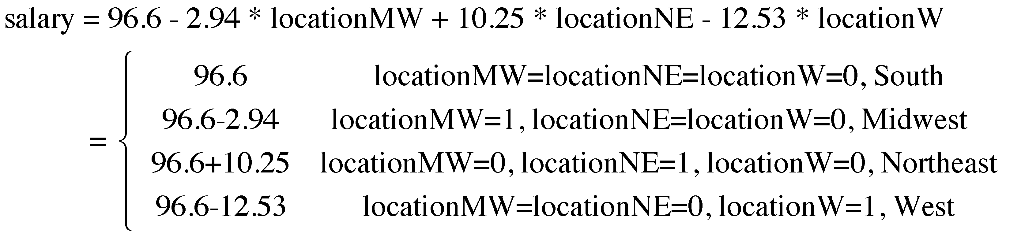
Based on the analysis, we can get the following information:
- The average salary of each area. The South area is the reference area, called reference group since the other groups can be directly compared with it.
-2.94is the difference in the average salaries between South and Midwest. Whether this difference is significantly different from 0 can be tested, therefore, through testing the regression coefficient oflocationMW. Sincet = -1.073, p = 0.287, the difference is not signifcant at the 0.05 level.10.25is the difference in the average salaries between South and Northeast. Sincet = 3.995, p = .0001for the parameter in the regression, the difference is significantly different from 0.-12.53is the difference in the average salaries between South and West. Sincet = -4.686, p = 1.11e-05for the parameter in the regression, the difference is significantly different from 0.
Testing the significance of the predictor
To test the significance of a categorical predictor, one can check the overall model fit of the regression analysis based on the F-test. This is equivalent to test the significance of all the dummy variables together. For this specific example, we have F=27.51 and p-value=2.287e-12. Therefore, the predictor is statistically significant.
Example 3. Two categorical predictors (two-way ANOVA)
Now let's consider the use of both predictors: public and location. With two categorical variables, we can dummy code each of them separately. Then, we should combine the dummy coded variables together to identify features based on the predictors for all possible subjects in the data. For example, for the current analysis, we have the following 4 dummy coded variables.
| Sector | Location | MW | NE | W | Public |
| Public | South | 0 | 0 | 0 | 1 |
| Public | Midwest | 1 | 0 | 0 | 1 |
| Public | Northeast | 0 | 1 | 0 | 1 |
| Public | West | 0 | 0 | 1 | 1 |
| Private | South | 0 | 0 | 0 | 0 |
| Private | Midwest | 1 | 0 | 0 | 0 |
| Private | Northeast | 0 | 1 | 0 | 0 |
| Private | West | 0 | 0 | 1 | 0 |
In fitting the model, we would expect the three dummy variables locationMW, locationNE, locationW for the categorical variable location and publicPublic for the categorical variable public. Note that when locationMW=0, locationNE=0, locationW=0 and publicPublic=1, the college is a public college in the south. For the other colleges, they can be identified in the same way using the 4 dummy coded variables.
The R input and output for the analysis are given below.
> usedata('college'); attach(college)
> salary <- salary / 1000
>
> public<-factor(public, c(0,1), labels=c('Private', 'Public'))
> location<-factor(location, c(1,2,3,4), labels=c('S', 'MW','NE', 'W'))
>
> summary(lm(salary~public+location))

Call:
lm(formula = salary ~ public + location)

Residuals:
    Min      1Q  Median      3Q     Max
-17.147  -4.754  -0.348   2.847  31.672

Coefficients:
             Estimate Std. Error t value Pr(>|t|)
(Intercept)    99.556      1.904  52.296  < 2e-16 ***
publicPublic   -7.301      1.828  -3.994 0.000143 ***
locationMW     -2.402      2.522  -0.953 0.343662
locationNE      8.793      2.386   3.685 0.000415 ***
locationW     -10.926      2.488  -4.391 3.42e-05 ***
---
Signif. codes:  0 '***' 0.001 '**' 0.01 '*' 0.05 '.' 0.1 ' ' 1

Residual standard error: 7.86 on 80 degrees of freedom
Multiple R-squared:  0.587,	Adjusted R-squared:  0.5664
F-statistic: 28.43 on 4 and 80 DF,  p-value: 1.06e-14

>
Based on the output, we can calculate the expected salary for each type of college as below:
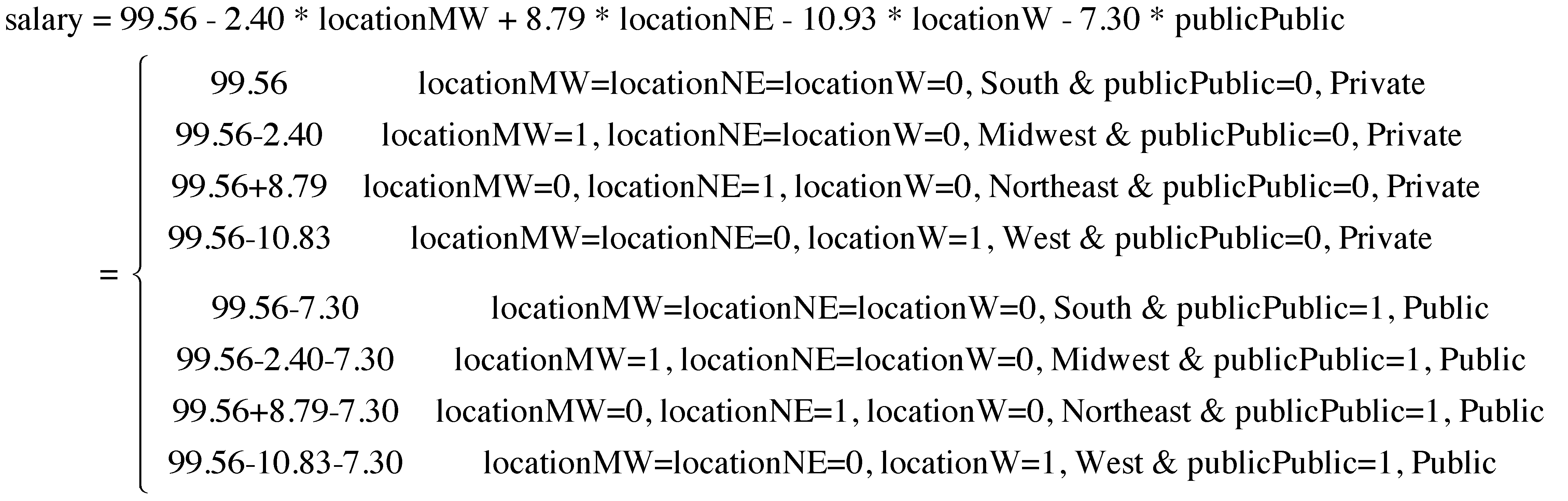
With this, we can easily calculate the difference in salary between any two types of colleges.
Testing the significance of the predictor
Note to test the significance of public variable, we can directly look at the coefficient for publicPublic since there is only one dummy variable here. For this example, it is significant given t=-3.994 with a p-value=0.00014.
For testing the significance of location, it is equivalent to test the significance of a subset of coefficients for the three dummy variables related to location. In the case, we can compare two models, one with both categorical predictors and the other with public predictor only. Then we can conduct a F-test for comparing the two models. From the comparison, we have an F = 21.887 with a p-value = 1.908e-10. Therefore, location is significant above and beyond the predictor public.
> usedata('college'); attach(college)
> salary <- salary / 1000
>
> public<-factor(public, c(0,1), labels=c('Private', 'Public'))
> location<-factor(location, c(1,2,3,4), labels=c('S', 'MW','NE', 'W'))
>
> m1 <- lm(salary~public+location)
> m2 <- lm(salary~public)
> anova(m2,m1)
Analysis of Variance Table

Model 1: salary ~ public
Model 2: salary ~ public + location
  Res.Df    RSS Df Sum of Sq      F    Pr(>F)
1     83 9000.1
2     80 4943.0  3    4057.1 21.887 1.908e-10 ***
---
Signif. codes:  0 '***' 0.001 '**' 0.01 '*' 0.05 '.' 0.1 ' ' 1
>
Example 4. Two categorical predictors with interaction
We can also look the interaction effects between two categorical predictors. In doing the analysis, we simply include the product of the two predictors. R automatically includes the interaction terms among the dummy coded variables. To investigate the significance of the interaction, we similarly can compare the models with and without the interaction term. For this particular example, we have an F = 8.4569 with a p-value = 6.316e-05. Therefore, the interaction is significant.
> usedata('college'); attach(college)
> salary <- salary / 1000
>
> public<-factor(public, c(0,1), labels=c('Private', 'Public'))
> location<-factor(location, c(1,2,3,4), labels=c('S', 'MW','NE', 'W'))
>
> m1 <- lm(salary~public+location)
> m2 <- lm(salary~public*location)
> anova(m1,m2)
Analysis of Variance Table

Model 1: salary ~ public + location
Model 2: salary ~ public * location
  Res.Df  RSS Df Sum of Sq      F    Pr(>F)
1     80 4943
2     77 3718  3      1225 8.4569 6.316e-05 ***
---
Signif. codes:  0 '***' 0.001 '**' 0.01 '*' 0.05 '.' 0.1 ' ' 1
>
Note that one can directly apply anova() function in the regression analysis as in ANOVA.
Example 4. Regression with one categorical and one continuous predictors (ANCOVA)
One might argue that the salary is related to the cost of education. Therefore, when looking at the salary difference across locations, one should first control the effect of the cost of eduction. Such analysis can be carried out conveniently as below. And from the output, we still observe significant location effect after controlling the cost of eduction.
> usedata('college'); attach(college)
> salary <- salary / 1000
>
> public<-factor(public, c(0,1), labels=c('Private', 'Public'))
> location<-factor(location, c(1,2,3,4), labels=c('S', 'MW','NE', 'W'))
>
> cost <- cost/1000
> summary(res<-lm(salary~cost + location))

Call:
lm(formula = salary ~ cost + location)

Residuals:
     Min       1Q   Median       3Q      Max
-20.2444  -4.9326  -0.5719   3.1620  29.9388

Coefficients:
             Estimate Std. Error t value Pr(>|t|)
(Intercept)  87.78906    3.09770  28.340  < 2e-16 ***
cost          0.06052    0.01728   3.501  0.00076 ***
locationMW   -2.80035    2.56841  -1.090  0.27885
locationNE    9.23247    2.42247   3.811  0.00027 ***
locationW   -10.52177    2.56915  -4.095  0.00010 ***
---
Signif. codes:  0 '***' 0.001 '**' 0.01 '*' 0.05 '.' 0.1 ' ' 1

Residual standard error: 8.016 on 80 degrees of freedom
Multiple R-squared:  0.5705,	Adjusted R-squared:  0.549
F-statistic: 26.57 on 4 and 80 DF,  p-value: 4.956e-14

> anova(res)
Analysis of Variance Table

Response: salary
          Df Sum Sq Mean Sq F value    Pr(>F)
cost       1 2757.0 2756.97  42.903 5.120e-09 ***
location   3 4071.8 1357.26  21.121 3.571e-10 ***
Residuals 80 5140.8   64.26
---
Signif. codes:  0 '***' 0.001 '**' 0.01 '*' 0.05 '.' 0.1 ' ' 1
>
Post-hoc comparison
Given the above regression analysis, we can conclude that the location of a university and the private/public sector of the university are related to the average salary the students in the university earn. We can further compare, for example, a private midwest university with a public west university. To make such a comparison, we use the function contrast() in the package contrast. For example, based on the analysis below, students from public Western colleges earn significantly less than students from private Midwest colleges. Note that in using the function, we use a list() to tell the categories of each predictor in the comparison. Keep in mind that this kind of comparison can run into multiple comparison problem and therefore Bonferroni correction should be considered.
> usedata('college'); attach(college)
> salary <- salary / 1000
>
> public<-factor(public, c(0,1), labels=c('Private', 'Public'))
> location<-factor(location, c(1,2,3,4), labels=c('S', 'MW','NE', 'W'))
>
> m1 <- lm(salary~public+location)
>
> library(contrast)
Loading required package: rms
Loading required package: Hmisc
Loading required package: lattice
Loading required package: survival
Loading required package: Formula
Loading required package: ggplot2

Attaching package: 'Hmisc'

The following objects are masked from 'package:base':

    format.pval, round.POSIXt, trunc.POSIXt, units

Loading required package: SparseM

Attaching package: 'SparseM'

The following object is masked from 'package:base':

    backsolve

> contrast(m1, list(location='W', public='Public'),
+              list(location='MW', public='Private'))
lm model parameter contrast

   Contrast    S.E.     Lower    Upper     t df Pr(>|t|)
1 -15.82522 2.93855 -21.67312 -9.97732 -5.39 80        0
>
To cite the book, use:
Zhang, Z. & Wang, L. (2017-2026). Advanced statistics using R. Granger, IN: ISDSA Press. https://doi.org/10.35566/advstats. ISBN: 978-1-946728-01-2.
To take the full advantage of the book such as running analysis within your web browser, please subscribe.