
Confirmatory Factor Analysis
Exploratory factor analysis can be used to identify common factors and factor structure among a set of observed variables / indicators. Confirmatory factor analysis (CFA) can be used to study how well a hypothesized factor model fits a new sample from the same population or a sample from a different population. The CFA model is the same as the EFA model with the exception that restrictions can be placed on factor loadings, variances, covariances, and residual variances resulting in a more parsimonious model. Using CFA, one can
- investigate if a factor model fits a new sample from the same population – the confirmatory aspect.
- evaluate if a factor model fits a sample from a different population – measurement invariance,
- study the behavior of new measurement items embedded in a previously studied measurement instrument, and
- estimate factor scores.
An example
The study by Karl J. Holzinger and Frances Swineford involves data collection from two schools, the Grant-White School (\(n=145\)) and Pasteur School (\(n=156\)). In the EFA example, we have identified 4 factors with data from the the Grant-White School. We now investigate whether the same factor model would fit the data in the Pasteur School. The data are saved in the file Pasteur.csv.
Confirmatory factor analysis
The model
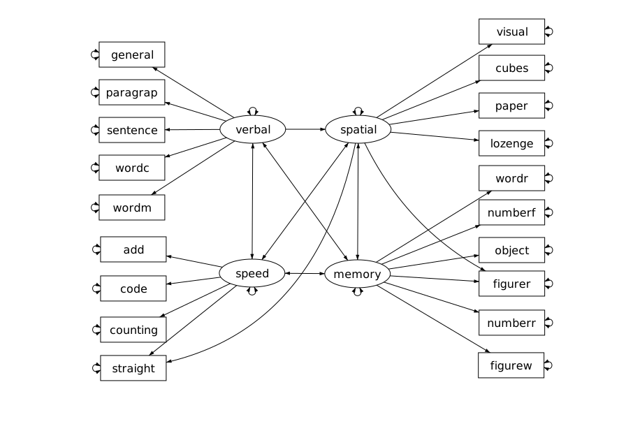
The path diagram for the model is given in the figure below. Note that we have assumed there are 4 factors. And the indicators of each factor are also known. This model is based on the EFA of Grant-White school data with the factor loadings greater than 0.3 kept in the model.
Model estimation
To estimate a confirmatory factor model, the R package lavaan can used. A confirmatory factor model cannot be identified without proper constraints, that's, to fix some parameters to be known values in the model. The reason is that factors are unmeasured and thus have no scales. To identify a model, the factors have to be given specific scales. There are two ways to do this. First, we can fix the variance of a factor to be 1. This is to standardize the factor. Second, we can fix the loading of one observed variable or indicator to be one. This is essentially to make the factor to have the same scale as the observed variables. Fixing a factor loading or a factor variance is the minimum requirement to identify a factor model. However, this does not guarantee a model is identifiable. Practically, if a model cannot be identified, the software used to estimate the model will not run correctly.
The cfa() function in lavaan can be used to estimate a factor model. To use the function, we need to first specify the factor model. A factor model take the format
factor =~ y1 + y2 +y3
Note that we use the symbol "=~" to define a factor. The factor is on the left of the symbol and the indicators are on the right of it.
The R code for the example is given below.
> library(lavaan)
This is lavaan 0.5-23.1097
lavaan is BETA software! Please report any bugs.
> usedata('Pasteur.csv')
>
> cfa.model<-'
+ spatial =~ visual+cubes+paper+lozenge+straight+figurer
+ verbal =~ general+paragrap+sentence+wordc+wordm
+ speed =~ add+code+counting+straight
+ memory =~ wordr+numberr+figurer+object+numberf+figurew
+ '
>
> cfa.est<-cfa(cfa.model, data=Pasteur)
> summary(cfa.est, fit=TRUE)
lavaan (0.5-23.1097) converged normally after 251 iterations

  Number of observations                           156

  Estimator                                         ML
  Minimum Function Test Statistic              238.751
  Degrees of freedom                               144
  P-value (Chi-square)                           0.000

Model test baseline model:

  Minimum Function Test Statistic             1149.278
  Degrees of freedom                               171
  P-value                                        0.000

User model versus baseline model:

  Comparative Fit Index (CFI)                    0.903
  Tucker-Lewis Index (TLI)                       0.885

Loglikelihood and Information Criteria:

  Loglikelihood user model (H0)              -9899.892
  Loglikelihood unrestricted model (H1)      -9780.517

  Number of free parameters                         46
  Akaike (AIC)                               19891.785
  Bayesian (BIC)                             20032.078
  Sample-size adjusted Bayesian (BIC)        19886.474

Root Mean Square Error of Approximation:

  RMSEA                                          0.065
  90 Percent Confidence Interval          0.050  0.079
  P-value RMSEA <= 0.05                          0.050

Standardized Root Mean Square Residual:

  SRMR                                           0.079

Parameter Estimates:

  Information                                 Expected
  Standard Errors                             Standard

Latent Variables:
                   Estimate  Std.Err  z-value  P(>|z|)
  spatial =~
    visual            1.000
    cubes             0.396    0.089    4.465    0.000
    paper             0.233    0.051    4.547    0.000
    lozenge           1.087    0.182    5.961    0.000
    straight          1.599    0.623    2.567    0.010
    figurer           0.535    0.139    3.836    0.000
  verbal =~
    general           1.000
    paragrap          0.282    0.024   11.846    0.000
    sentence          0.463    0.035   13.322    0.000
    wordc             0.388    0.038   10.177    0.000
    wordm             0.589    0.047   12.585    0.000
  speed =~
    add               1.000
    code              0.835    0.145    5.758    0.000
    counting          0.708    0.147    4.811    0.000
    straight          1.091    0.265    4.115    0.000
  memory =~
    wordr             1.000
    numberr           0.537    0.106    5.040    0.000
    figurer           0.486    0.106    4.570    0.000
    object            0.379    0.070    5.372    0.000
    numberf           0.277    0.060    4.638    0.000
    figurew           0.245    0.055    4.444    0.000

Covariances:
                   Estimate  Std.Err  z-value  P(>|z|)
  spatial ~~
    verbal           21.927    5.770    3.800    0.000
    speed            24.531    9.382    2.615    0.009
    memory           10.542    4.998    2.109    0.035
  verbal ~~
    speed            66.093   17.349    3.810    0.000
    memory           10.027    7.727    1.298    0.194
  speed ~~
    memory           47.001   14.950    3.144    0.002

Variances:
                   Estimate  Std.Err  z-value  P(>|z|)
   .visual           21.376    4.533    4.716    0.000
   .cubes            19.547    2.401    8.139    0.000
   .paper             6.472    0.799    8.102    0.000
   .lozenge          52.062    7.715    6.748    0.000
   .straight        875.004  110.732    7.902    0.000
   .figurer          40.094    5.568    7.200    0.000
   .general          41.308    5.979    6.909    0.000
   .paragrap          4.185    0.571    7.330    0.000
   .sentence          6.615    1.058    6.252    0.000
   .wordc            13.215    1.664    7.943    0.000
   .wordm            14.218    2.063    6.892    0.000
   .add             415.730   55.840    7.445    0.000
   .code             75.538   19.745    3.826    0.000
   .counting        280.324   35.795    7.831    0.000
   .wordr            83.348   12.917    6.452    0.000
   .numberr          43.595    5.790    7.529    0.000
   .object           16.578    2.329    7.119    0.000
   .numberf          15.587    1.982    7.865    0.000
   .figurew          14.000    1.752    7.989    0.000
    spatial          28.852    6.417    4.496    0.000
    verbal           96.582   15.354    6.290    0.000
    speed           200.381   59.608    3.362    0.001
    memory           60.814   15.974    3.807    0.000

>
Output
By default, the cfa() function fixes a factor loading for each factor to be 1 and estimates the rest factor loadings. Different from EFA, CFA also test the significance of the factor loadings based on a z-test. For example, the factor loading for cubes on factor 1 is 0.396 with the standard error 0.089. The corresponding z-value is 4.465 with a p-value almost 0. Therefore, this factor loading is statistically significant from 0. In addition, it also estimates the factor variances and covariances as well as the uniqueness factor variances.
Model fit evaluation
CFA provides a lot more information to evaluate whether a model fits a sample. First, a chi-square test can be used. For this test, the null hypothesis is that the model fits the data well. Therefore, one would hope to get a small chi-square statistic and a corresponding large p-value. Typically, when p-value is larger than 0.5, one fails to reject the model.
There are many other fit statistics and indices that can be used to evaluate model fit. The most widely used ones include CFI, RMSEA, and SRMR.
- Comparative fit index (CFI) compares the model under evaluation with a baseline model. One form of the baseline model is the independent model where it assumes the independence among the observed variables. In general, such a baseline model would not fit the data well. Therefore, CFI measures the relative improvement of the current model. It is generally accepted that a CFI greater than 0.96 (or 0.95) indicates a good fit model.
- Root mean square error of approximation (RMSEA) is a measure of chi-square attributed to each participate after controlling the model complexity. Therefore, a smaller value indicates better fit. In the literature,
- a RMSEA $\leq 0.05$ indicates a model fits the data closely.
- a $0.05<$ RMSEA $\leq 0.08$ indicates a model fits the data reasonably well.
- a RMSEA $>0.1$ indicates a model is a bad model.
- Standardized root mean square residual (SRMR) measures the difference between the observed covariance matrix from the data and the predicted covariance matrix based on the model. A value SRMR=0 indicates a perfect of the model. In general, a value less than 0.08 is considered a good fit of the model under evaluation.
Using these criteria, we can evaluate whether the confirmatory factor model identified using the data from Grant-White school fits the data from the Pasteur school well.
- The chi-square statistic (
Minimum Function Test Statisticin the output) is 238.75 with the degrees of freedom 144 and a p-value close to 0. Therefore, one would reject the hypothesis that the model fits the data simply based on it. - Comparative Fit Index (CFI) is 0.903, which is smaller than the cut-off value 0.95. It also suggests a bad fit.
- The RMSEA = 0.065, which lies the range of a reasonable fit model.
- The SRMR = 0.079, which is smaller than but close to the cut-off value 0.08.
Overall, the chi-square test and the other criteria suggest the model barely fits the data. Therefore, we cannot replicate the factor structure identified in EFA for the Grant-White school data in the Pasteur school.
Estimate the model with standardized factors
Instead of fitting a factor loading to be 1, we can also fix the factor variances to be 1. The R code below does the analysis. Note that the model fit is exactly the same as before. However, we can now directly estimate the factor correlation matrix.
> library(lavaan)
This is lavaan 0.5-23.1097
lavaan is BETA software! Please report any bugs.
> usedata('Pasteur.csv')
>
> cfa.model<-'
+ spatial =~ visual+cubes+paper+lozenge+straight+figurer
+ verbal =~ general+paragrap+sentence+wordc+wordm
+ speed =~ add+code+counting+straight
+ memory =~ wordr+numberr+figurer+object+numberf+figurew
+ '
>
> cfa.est<-cfa(cfa.model, data=Pasteur, std.lv=TRUE)
> summary(cfa.est, fit=TRUE)
lavaan (0.5-23.1097) converged normally after 191 iterations

  Number of observations                           156

  Estimator                                         ML
  Minimum Function Test Statistic              238.751
  Degrees of freedom                               144
  P-value (Chi-square)                           0.000

Model test baseline model:

  Minimum Function Test Statistic             1149.278
  Degrees of freedom                               171
  P-value                                        0.000

User model versus baseline model:

  Comparative Fit Index (CFI)                    0.903
  Tucker-Lewis Index (TLI)                       0.885

Loglikelihood and Information Criteria:

  Loglikelihood user model (H0)              -9899.892
  Loglikelihood unrestricted model (H1)      -9780.517

  Number of free parameters                         46
  Akaike (AIC)                               19891.785
  Bayesian (BIC)                             20032.078
  Sample-size adjusted Bayesian (BIC)        19886.474

Root Mean Square Error of Approximation:

  RMSEA                                          0.065
  90 Percent Confidence Interval          0.050  0.079
  P-value RMSEA <= 0.05                          0.050

Standardized Root Mean Square Residual:

  SRMR                                           0.079

Parameter Estimates:

  Information                                 Expected
  Standard Errors                             Standard

Latent Variables:
                   Estimate  Std.Err  z-value  P(>|z|)
  spatial =~
    visual            5.371    0.597    8.993    0.000
    cubes             2.124    0.433    4.901    0.000
    paper             1.254    0.250    5.012    0.000
    lozenge           5.837    0.790    7.385    0.000
    straight          8.589    3.240    2.651    0.008
    figurer           2.872    0.697    4.121    0.000
  verbal =~
    general           9.828    0.781   12.580    0.000
    paragrap          2.773    0.234   11.850    0.000
    sentence          4.551    0.340   13.389    0.000
    wordc             3.811    0.375   10.172    0.000
    wordm             5.790    0.459   12.605    0.000
  speed =~
    add              14.156    2.105    6.723    0.000
    code             11.823    1.224    9.658    0.000
    counting         10.024    1.673    5.990    0.000
    straight         15.440    3.235    4.773    0.000
  memory =~
    wordr             7.798    1.024    7.614    0.000
    numberr           4.185    0.683    6.129    0.000
    figurer           3.790    0.707    5.363    0.000
    object            2.953    0.434    6.798    0.000
    numberf           2.160    0.398    5.428    0.000
    figurew           1.913    0.374    5.121    0.000

Covariances:
                   Estimate  Std.Err  z-value  P(>|z|)
  spatial ~~
    verbal            0.415    0.085    4.895    0.000
    speed             0.323    0.103    3.129    0.002
    memory            0.252    0.109    2.303    0.021
  verbal ~~
    speed             0.475    0.081    5.902    0.000
    memory            0.131    0.098    1.336    0.181
  speed ~~
    memory            0.426    0.097    4.410    0.000

Variances:
                   Estimate  Std.Err  z-value  P(>|z|)
   .visual           21.376    4.533    4.716    0.000
   .cubes            19.547    2.401    8.139    0.000
   .paper             6.472    0.799    8.102    0.000
   .lozenge          52.062    7.715    6.748    0.000
   .straight        875.006  110.732    7.902    0.000
   .figurer          40.093    5.568    7.200    0.000
   .general          41.308    5.979    6.909    0.000
   .paragrap          4.185    0.571    7.330    0.000
   .sentence          6.615    1.058    6.252    0.000
   .wordc            13.215    1.664    7.943    0.000
   .wordm            14.218    2.063    6.892    0.000
   .add             415.731   55.841    7.445    0.000
   .code             75.538   19.745    3.826    0.000
   .counting        280.324   35.795    7.831    0.000
   .wordr            83.347   12.917    6.452    0.000
   .numberr          43.595    5.790    7.529    0.000
   .object           16.578    2.329    7.119    0.000
   .numberf          15.587    1.982    7.865    0.000
   .figurew          14.000    1.752    7.989    0.000
    spatial           1.000
    verbal            1.000
    speed             1.000
    memory            1.000

>
To cite the book, use:
Zhang, Z. & Wang, L. (2017-2026). Advanced statistics using R. Granger, IN: ISDSA Press. https://doi.org/10.35566/advstats. ISBN: 978-1-946728-01-2.
To take the full advantage of the book such as running analysis within your web browser, please subscribe.