In the ACTIVE study, we have data on verbal ability at two times (hvltt and hvltt2). To investigate the relationship between them, we can generate a scatterplot using hvltt and hvltt2 as shown below. From the plot, it is easy to observe that those with a higher score on hvltt tend to have a higher score on hvltt2. Certainly, it is not difficult to find two people where the one with higher score on hvltt has a lower score on hvltt2. But in general hvltt and hvltt2 tend to go up and down together.
Furthermore, the association between hvltt and hvltt2 seems to be able to be described by a straight line. The red line in the figure is one that run across the points in the scatter plot. The straight line can be expressed using
\[hvltt2 = 5.19 + 0.73*hvltt\]
It says multiplying one's test score (hvltt) at the first occasion by 0.73 and adding 5.19 predict his/her test score (hvltt2) at the second occasion.
>>> import pandas as pd
>>> active = pd.read_csv("https://advstats.psychstat.org/data/active.csv")
>>>
>>> import seaborn as sns
>>> import matplotlib.pyplot as plt
>>>
>>> # Create scatterplot
>>> sns.regplot(x='hvltt', y='hvltt2', color='blue', data=active)

>>>
>>> # Add labels and title
>>> plt.title('Scatterplot using Seaborn')
Text(0.5, 1.0, 'Scatterplot using Seaborn')
>>> plt.xlabel('Verbal test score at time 1')
Text(0.5, 0, 'Verbal test score at time 1')
>>> plt.ylabel('Verbal test score at time 2')
Text(0, 0.5, 'Verbal test score at time 2')
>>>
>>> plt.savefig('scatter.svg', format='svg')
>>> # Show the plot
>>> plt.show()
Simple regression model
A regression model / regression analysis can be used to predict the value of one variable (the dependent or outcome variable) on the basis of other variables (the independent and predictor variables). Typically, we use \(y\) to denote the dependent variable and \(x\) to denote an independent variable.
The simple linear regression model for the population can be written as
\[y = \beta_0 + \beta_1 x + \epsilon\]
where
\(\beta_0\) is called the intercept, which is also the average value of \(y\) when \(x=0\).
\(\beta_1\) is called the slope, which is the change in \(y\) given the unit change in \(x\). Therefore, it is also called rate of change.
\(\epsilon\) is a normal error that is often assumed to have a normal distribution with mean 0 and unknown variance \(\sigma^2\). This term represents the part of information in \(y\) that cannot be explained by \(x\).
Parameter estimation
In practice, the population parameters $\beta_0$ and $\beta_1$ are unknown. However, with a set of sample data, they can be estimated. One often used estimation method for regression analysis is called least squares estimation method. We explain the method here.
Let the model below represent the estimated regression model:
\[ y = b_0 + b_1 x + e \]
where
\(b_0\) is an estimate of the population intercept \(\beta_0\)
\(b_1\) is an estimate of the population slope \(\beta_1\)
\(e\) is the residual, which estimate \(\epsilon\).
Assume we already get the estimates \(b_0\) and \(b_1\), then we can make a prediction of the value of \(y\) based on the value of \(x\). For example, for the \(i\)th participant, if his/her score on the independent variable is \(x_i\), then the corresponding predicted outcome \(\hat{y}_i\) based on the regression model is
\[\hat{y}_i = b_0 + b_1 x_i.\]
The difference between the predicted value and the observed data for this participant, also called the prediction error, is
\(e_i = y_i - \hat{y}_i\).
The parameter \(b_0\) and \(b_1\) potentially can take any values. A good choice could be those that make the errors smallest, which leads to the least squares estimation.
Least squares estimation
The least squares estimation obtains \(b_0\) and \(b_1\) by minimizing the sum of the squared prediction errors. Therefore, such a set of parameters makes \(\hat{y}_i\) closest to \(y_i\) on average. Specifically, one minimizes SSE as
where \(\bar{x} = \sum_{i=1}^{n} x_i / n\) and \(\bar{y} = \sum_{i=1}^{n} y_i / n\).
Hypothesis testing
If no linear relationship exists between the two variables, we would expect the regression line to be horizontal, that is, to have a slope of zero. Therefore, we can test whether the hypothesis that the population regression slope is 0. More specifically, we have the null hypothesis
\[ H_0: \beta_1 = 0.\]
And the alternative hypothesis is
\[ H_1: \beta_1 \neq 0.\]
To conduct the hypothesis testing, we calculate a t test statistic
\[ t = \frac{b_1 - \beta_1}{s_{b_1}} \]
where \(s_{b_1}\) is the standard error of \(b_1\).
If \(\beta_1 = 0\) in the population, then the statistic t follows a t-distribution with degrees of freedom \(n-2\).
Regression in python
Both the parameter estimates and the t test can be conducted using the statsmodels library.
An example
To show how to conduct a simple linear regression, we analyze the relationship between hvltt and hvltt2 from the ACTIVE study. The input and output for the regression analysis is given below.
The function OLS can be used, which takes the y and x data. Note that the design matrix x needs to have a constant. The constant can be added using the add_constant function.
The model is specfifed using the OLS() function and is estimated using the fit() function
For more detailed results, the summary() function can be applied to the regression object.
The estimated intercept is 5.1853 and the estimated slope is 0.7342. Their corresponding standard errors are 0.5463 and 0.200, respectively.
For testing the hypothesis that the slope is 0 -- \(H_0: \beta_1 = 0\). The t-statistic is 36.719. Based on the t distribution with the degrees of freedom 1573, we have the p-value < 2e-16. Therefore, one would reject the null hypothesis if the signifance level 0.05 is used.
Similarly, for testing the hypothesis that the intercept is 0 -- \(H_0: \beta_0 = 0\). The t-statistic is 9.492. Based on the t distribution with the degrees of freedom 1573, we have the p-value < 2e-16. Therefore, one would reject the null hypothesis.
>>> import pandas as pd
>>> active = pd.read_csv("https://advstats.psychstat.org/data/active.csv")
>>>
>>> import statsmodels.api as sm
>>>
>>> ## get data for y & x
>>> y = active['hvltt2']
>>>
>>> ## add a column of 1 to x
>>> x = active['hvltt']
>>> x = sm.add_constant(x)
>>> x.head()
   const  hvltt
0    1.0     28
1    1.0     24
2    1.0     24
3    1.0     35
4    1.0     35
>>>
>>> ## specify the model
>>> model = sm.OLS(y, x)
>>>
>>> ## fit the model
>>> results = model.fit()
>>>
>>> ## print the results
>>> print(results.summary())
                            OLS Regression Results
==============================================================================
Dep. Variable:                 hvltt2   R-squared:                       0.462
Model:                            OLS   Adj. R-squared:                  0.461
Method:                 Least Squares   F-statistic:                     1348.
Date:                Sun, 24 Nov 2024   Prob (F-statistic):          1.06e-213
Time:                        14:20:54   Log-Likelihood:                -4397.7
No. Observations:                1575   AIC:                             8799.
Df Residuals:                    1573   BIC:                             8810.
Df Model:                           1
Covariance Type:            nonrobust
==============================================================================
                 coef    std err          t      P>|t|      [0.025      0.975]
------------------------------------------------------------------------------
const          5.1854      0.546      9.492      0.000       4.114       6.257
hvltt          0.7342      0.020     36.719      0.000       0.695       0.773
==============================================================================
Omnibus:                        9.905   Durbin-Watson:                   2.040
Prob(Omnibus):                  0.007   Jarque-Bera (JB):                9.877
Skew:                          -0.188   Prob(JB):                      0.00717
Kurtosis:                       3.099   Cond. No.                         150.
==============================================================================

Notes:
[1] Standard Errors assume that the covariance matrix of the errors is correctly specified.
>>>
>>> ## using formula
>>> import statsmodels.formula.api as smf
>>> test = smf.ols("hvltt2~hvltt", data=active).fit()
>>> print(test.summary())
                            OLS Regression Results
==============================================================================
Dep. Variable:                 hvltt2   R-squared:                       0.462
Model:                            OLS   Adj. R-squared:                  0.461
Method:                 Least Squares   F-statistic:                     1348.
Date:                Sun, 24 Nov 2024   Prob (F-statistic):          1.06e-213
Time:                        14:20:54   Log-Likelihood:                -4397.7
No. Observations:                1575   AIC:                             8799.
Df Residuals:                    1573   BIC:                             8810.
Df Model:                           1
Covariance Type:            nonrobust
==============================================================================
                 coef    std err          t      P>|t|      [0.025      0.975]
------------------------------------------------------------------------------
Intercept      5.1854      0.546      9.492      0.000       4.114       6.257
hvltt          0.7342      0.020     36.719      0.000       0.695       0.773
==============================================================================
Omnibus:                        9.905   Durbin-Watson:                   2.040
Prob(Omnibus):                  0.007   Jarque-Bera (JB):                9.877
Skew:                          -0.188   Prob(JB):                      0.00717
Kurtosis:                       3.099   Cond. No.                         150.
==============================================================================

Notes:
[1] Standard Errors assume that the covariance matrix of the errors is correctly specified.
>>>
>>> ## all attributes of the model
>>> print(dir(test))
['HC0_se', 'HC1_se', 'HC2_se', 'HC3_se', '_HCCM', '__class__', '__delattr__', '__dict__', '__dir__', '__doc__', '__eq__', '__format__', '__ge__', '__getattribute__', '__getstate__', '__gt__', '__hash__', '__init__', '__init_subclass__', '__le__', '__lt__', '__module__', '__ne__', '__new__', '__reduce__', '__reduce_ex__', '__repr__', '__setattr__', '__sizeof__', '__str__', '__subclasshook__', '__weakref__', '_abat_diagonal', '_cache', '_data_attr', '_data_in_cache', '_get_robustcov_results', '_get_wald_nonlinear', '_is_nested', '_transform_predict_exog', '_use_t', '_wexog_singular_values', 'aic', 'bic', 'bse', 'centered_tss', 'compare_f_test', 'compare_lm_test', 'compare_lr_test', 'condition_number', 'conf_int', 'conf_int_el', 'cov_HC0', 'cov_HC1', 'cov_HC2', 'cov_HC3', 'cov_kwds', 'cov_params', 'cov_type', 'df_model', 'df_resid', 'diagn', 'eigenvals', 'el_test', 'ess', 'f_pvalue', 'f_test', 'fittedvalues', 'fvalue', 'get_influence', 'get_prediction', 'get_robustcov_results', 'info_criteria', 'initialize', 'k_constant', 'llf', 'load', 'model', 'mse_model', 'mse_resid', 'mse_total', 'nobs', 'normalized_cov_params', 'outlier_test', 'params', 'predict', 'pvalues', 'remove_data', 'resid', 'resid_pearson', 'rsquared', 'rsquared_adj', 'save', 'scale', 'ssr', 'summary', 'summary2', 't_test', 't_test_pairwise', 'tvalues', 'uncentered_tss', 'use_t', 'wald_test', 'wald_test_terms', 'wresid']
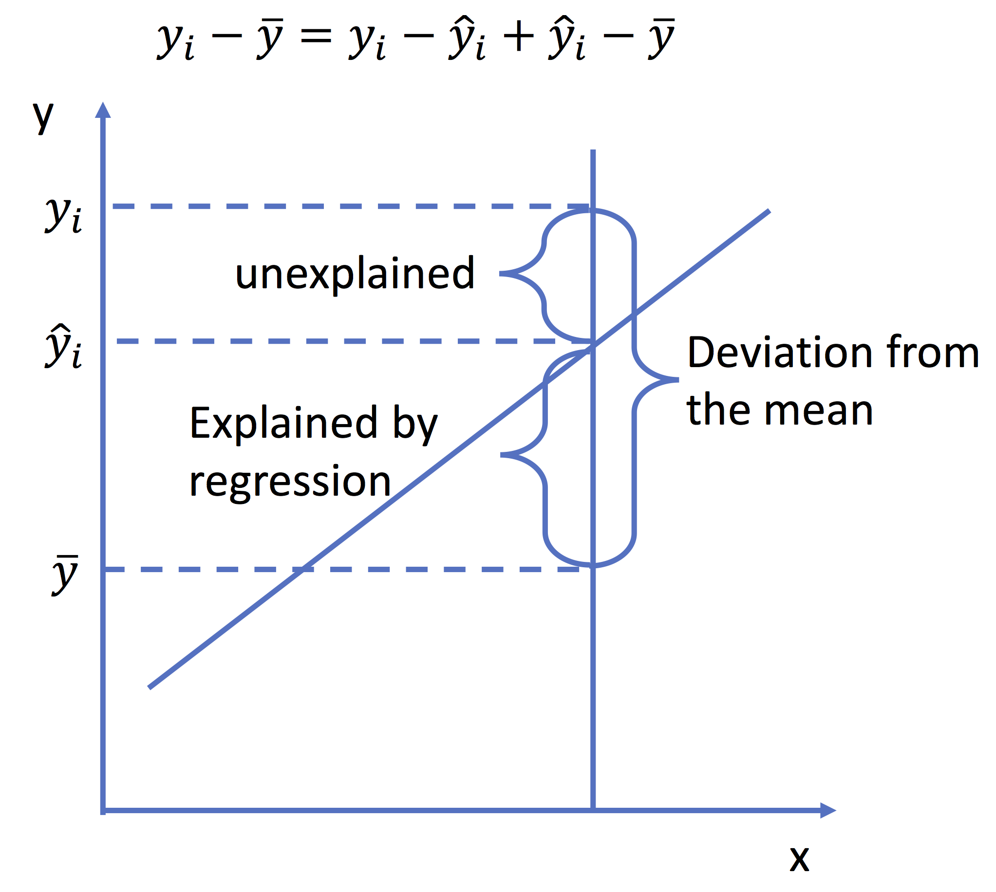
Coefficient of Determination (Multiple R-squared)
Significant tests show if a linear relationship exists but not the strength of the relationship. The coefficient of determination, \(R^2\), is a descriptive measure of the strength of the regression relationship, a measure on how well the regression line fits the data. In general the higher the value of \(R^2\), the better the model fits the data.
\(R^2 = 1\): Perfect match between the line and the data points.
\(R^2 = 0\): There are no linear relationship between x and y.
\(R^2\) is an effect size measure. Cohen (1988) defined some standards for interpreting \(R^2\).
\(R^2 = .01\): Small effect
\(R^2 = .06\): Medium effect
\(R^2 = .15\): Large effect.
For the regression example, the \(R^2 = 0.4615\), representing a large effect.
Calculation and interpretation of \(R^2\)
Simply speaking, the \(R^2\) tells the percentage of variance in \(y\) that can be explained by the regression model or by \(x\).
To cite the book, use:
Zhang, Z. & Wang, L. (2017-2026). Advanced statistics using R. Granger, IN: ISDSA Press. https://doi.org/10.35566/advstats. ISBN: 978-1-946728-01-2. To take the full advantage of the book such as running analysis within your web browser, please subscribe.