
Mediation Analysis
Path diagrams
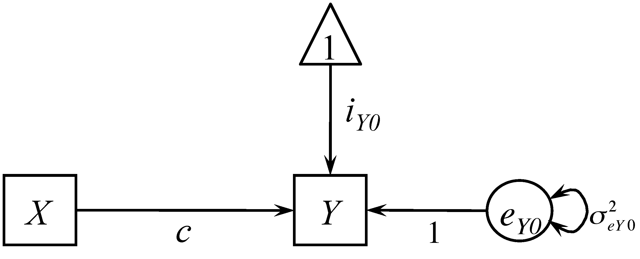
Consider a bivariate relationship between X and Y. If X is a predictor and Y is the outcome, we can fit a regression model
\[Y=i_{Y0}+cX+e_{Y0}\]
where $c$ is the effect of $X$ on $Y$, also called as the total effect of $X$ on $Y$. The model can be expressed as a path diagram as shown below.
Rules to draw a path diagram
In a path diagram, there are three types of shapes: a rectangle, a circle, and a triangle, as well as two types of arrows: one-headed (single-headed) arrow and two-headed (double-headed) arrows.
A rectangle represents an observed variable, which is a variable in the dataset with known information from the subjects. A circle or elliptical represents an unobserved variable, which can be the residuals, errors, or factors. A triangle, typically with 1 in it, represents either an intercept or a mean.
A one-headed arrow means that the variable on the side without the arrow predicts the variable on the side with the arrow. If the two-headed arrow is on a single variable, it represents a variance. If the two-headed arrow is between two variables, it represents the covariance between the two variables.
How to draw path diagrams?
Many different software can be used to draw path diagrams such as Powerpoint, Word, OmniGaffle, ect. For the ease of use, we recommend the online program WebSEM (https://websem.psychstat.org), which allows researchers to do SEM online, even on a smart phone. In addition, the drawn path diagram can be estimated using the uploaded/provided data (WebSEM). A simpler version of such program can be found at http://semdiag.psychstat.org.
What is mediation or what is a mediator?
In the classic paper on mediation analysis, Baron and Kenny (1986, p.1176) defined a mediator as "In general, a given variable may be said to function as a mediator to the extent that it accounts for the relation between the predictor and the criterion. " Therefore, mediation analysis answers the question why X can predict Y.
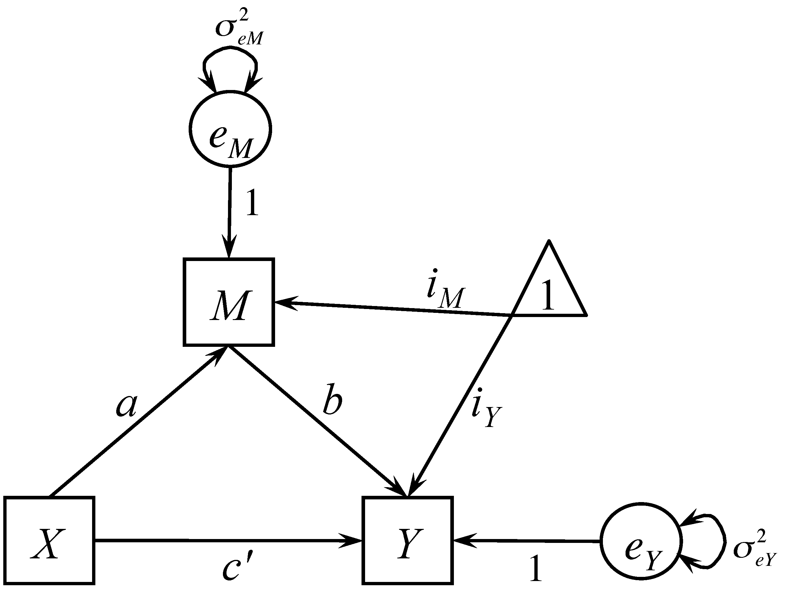
Suppose the effect of X on Y may be mediated by a mediating variable M. Then, we can write a mediation model as two regression equations
\begin{eqnarray*} M & = & i_{M}+aX+e_{M} \\ Y & = & i_{Y}+c'X+bM+e_{Y}. \end{eqnarray*}
This is the simplest but most popular mediation model. $c'$ is called the direct effect of X on Y with the inclusion of variable M. The indirect effect or mediation effect is $a*b$, the effect of X on Y through M. The total effect of X on Y is $c=c\prime+a*b$. This simple mediation model can also be portrayed as a path diagram shown below.
Note that a mediation model is a directional model. For example, the mediator is presumed to cause the outcome and not vice versa. If the presumed model is not correct, the results from the mediation analysis are of little value. Mediation is not defined statistically; rather statistics can be used to evaluate a presumed mediation model.
Mediation effects
The amount of mediation, which is called the indirect effect, is defined as the reduction of the effect of the input variable on the outcome, $c-c'$. $c-c' = ab$ when (1) multiple regression (or structural equation modeling without latent variables) is used, (2) there are no missing data, and (3) the same covariates are in the equations if there are any covariates. However, the two are only approximately equal for multilevel models, logistic analysis and structural equation models with latent variables. In this case, we calculate the total effect via $c'+ab$ instead of $c$. For the simplest mediation model without missing data, $ab=c-c'$.
Testing mediation effects
An example
We use the following example to show how to conduct mediation analysis and test mediation effects.
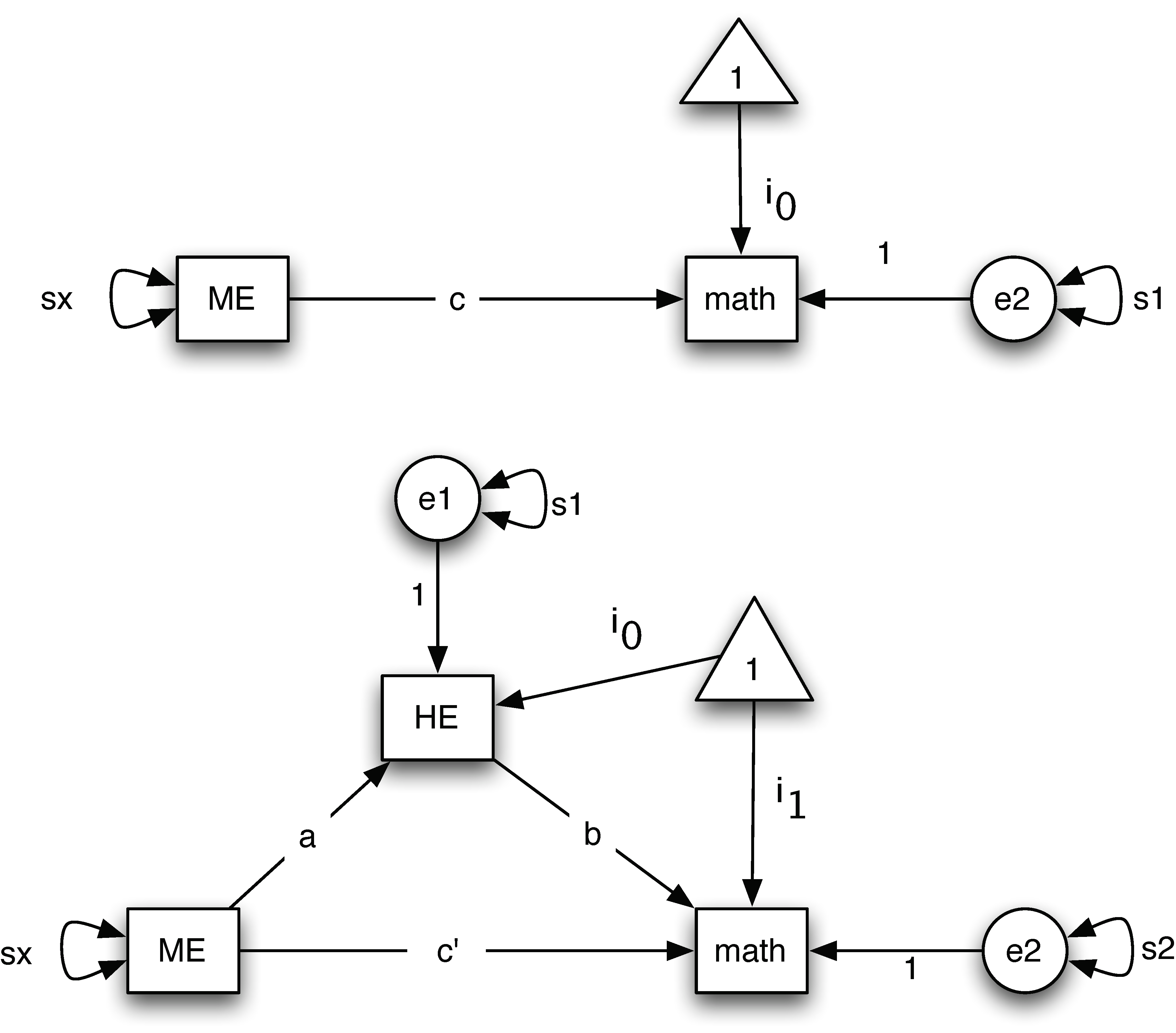
Research has found that parents' education levels can influence adolescent mathematics achievement directly and indirectly. For example, Davis-Kean (2005) showed that parents' education levels are related to children's academic achievement through parents' beliefs and behaviors. To test a similar hypothesis, we investigate whether home environment is a mediator in the relation between mothers' education and children's mathematical achievement. Data used in this example are from the National Longitudinal Survey of Youth, the 1979 cohort (NLSY79, for Human Resource Research, 2006). Data (nlsy.csv) were collected in 1986 from N=371 families on mothers' education level (ME), home environment (HE), and children's mathematical achievement (Math). For the mediation analysis, mothers' education is the input variable, home environment is the mediator, and children's mathematical achievement is the outcome variable. Using a path diagram, the involved mediation model is given below.
Baron and Kenny (1986) method
Baron and Kenny (1989) outlined a 4-step procedure to determine whether there is a mediation effect.
- Show that X is correlated with Y. Regress Y on X to estimate and test the path $c$. This step establishes that there is an effect that may be mediated.
- Show that X is correlated with M. Regress M on X to estimate and test path \(a\). This step essentially involves treating the mediator as if it were an outcome variable.
- Show that M affects Y. Regress Y on both X and M to estimate and test path \(b\). Note that it is not sufficient just to correlate the mediator with the outcome; the mediator and the outcome may be correlated because they are both caused by the input variable X. Thus, the input variable X must be controlled in establishing the effect of the mediator on the outcome.
- To establish that M completely mediates the X-Y relationship, the effect of X on Y controlling for M (path $c'$) should be zero. The effects in both Steps 3 and 4 are estimated in the same equation.
If all four of these steps are met, then the data are consistent with the hypothesis that variable M completely mediates the X-Y relationship, and if the first three steps are met but the Step 4 is not, then partial mediation is indicated.
The python code for the 4-step method for the example data is shown below.
>>> import pandas as pd
>>> nlsy = pd.read_csv('https://advstats.psychstat.org/data/nlsy.csv')
>>> nlsy.head()
   ME  HE  math
0  12   6     6
1  15   6    11
2   9   5     3
3   8   3     6
4   9   6    11
>>>
>>> ## Step 1: math ~ ME
>>> import statsmodels.formula.api as smf
>>> m1 = smf.ols("math ~ ME", data=nlsy).fit()
>>> print(m1.summary())
                            OLS Regression Results
==============================================================================
Dep. Variable:                   math   R-squared:                       0.050
Model:                            OLS   Adj. R-squared:                  0.047
Method:                 Least Squares   F-statistic:                     19.34
Date:                Mon, 25 Nov 2024   Prob (F-statistic):           1.43e-05
Time:                        21:41:37   Log-Likelihood:                -1093.0
No. Observations:                 371   AIC:                             2190.
Df Residuals:                     369   BIC:                             2198.
Df Model:                           1
Covariance Type:            nonrobust
==============================================================================
                 coef    std err          t      P>|t|      [0.025      0.975]
------------------------------------------------------------------------------
Intercept      6.1824      1.371      4.510      0.000       3.487       8.878
ME             0.5275      0.120      4.398      0.000       0.292       0.763
==============================================================================
Omnibus:                      112.662   Durbin-Watson:                   1.633
Prob(Omnibus):                  0.000   Jarque-Bera (JB):              537.431
Skew:                           1.212   Prob(JB):                    1.99e-117
Kurtosis:                       8.375   Cond. No.                         65.8
==============================================================================

Notes:
[1] Standard Errors assume that the covariance matrix of the errors is correctly specified.
>>>
>>> ## Step 2: HE ~ ME
>>> import statsmodels.formula.api as smf
>>> m2 = smf.ols("HE ~ ME", data=nlsy).fit()
>>> print(m2.summary())
                            OLS Regression Results
==============================================================================
Dep. Variable:                     HE   R-squared:                       0.028
Model:                            OLS   Adj. R-squared:                  0.025
Method:                 Least Squares   F-statistic:                     10.50
Date:                Mon, 25 Nov 2024   Prob (F-statistic):            0.00130
Time:                        21:41:37   Log-Likelihood:                -712.29
No. Observations:                 371   AIC:                             1429.
Df Residuals:                     369   BIC:                             1436.
Df Model:                           1
Covariance Type:            nonrobust
==============================================================================
                 coef    std err          t      P>|t|      [0.025      0.975]
------------------------------------------------------------------------------
Intercept      4.1094      0.491      8.365      0.000       3.143       5.075
ME             0.1393      0.043      3.240      0.001       0.055       0.224
==============================================================================
Omnibus:                       25.332   Durbin-Watson:                   1.881
Prob(Omnibus):                  0.000   Jarque-Bera (JB):               28.943
Skew:                          -0.682   Prob(JB):                     5.19e-07
Kurtosis:                       3.114   Cond. No.                         65.8
==============================================================================

Notes:
[1] Standard Errors assume that the covariance matrix of the errors is correctly specified.
>>>
>>> ## Step 3: math ~ ME + HE
>>> import statsmodels.formula.api as smf
>>> m3 = smf.ols("math ~ HE + ME", data=nlsy).fit()
>>> print(m3.summary())
                            OLS Regression Results
==============================================================================
Dep. Variable:                   math   R-squared:                       0.076
Model:                            OLS   Adj. R-squared:                  0.071
Method:                 Least Squares   F-statistic:                     15.16
Date:                Mon, 25 Nov 2024   Prob (F-statistic):           4.70e-07
Time:                        21:41:37   Log-Likelihood:                -1087.8
No. Observations:                 371   AIC:                             2182.
Df Residuals:                     368   BIC:                             2193.
Df Model:                           2
Covariance Type:            nonrobust
==============================================================================
                 coef    std err          t      P>|t|      [0.025      0.975]
------------------------------------------------------------------------------
Intercept      4.2736      1.476      2.895      0.004       1.370       7.177
HE             0.4645      0.143      3.238      0.001       0.182       0.747
ME             0.4628      0.120      3.853      0.000       0.227       0.699
==============================================================================
Omnibus:                      116.643   Durbin-Watson:                   1.620
Prob(Omnibus):                  0.000   Jarque-Bera (JB):              560.290
Skew:                           1.259   Prob(JB):                    2.16e-122
Kurtosis:                       8.469   Cond. No.                         80.1
==============================================================================

Notes:
[1] Standard Errors assume that the covariance matrix of the errors is correctly specified.
In Step 1, we fit a regression model using ME as the predictor and math as the outcome variable. Based on this analysis, we have $\hat{c}$ =.5275 (t = 4.298, p <.001) and thus ME is significantly related to math. Therefore, Step 1 is met: the input variable is correlated with the outcome.
In Step 2, we fit a regression model using ME as the predictor and HE as the outcome variable. From this analysis, we have $\hat{a}$ = .139 (t = 3.24, p = .0013) and thus ME is significantly related to HE. Therefore, Step 2 is met: the input variable is correlated with the mediator.
In Step 3, we fit a multiple regression model with ME and HE as predictors and math as the outcome variable. For the analysis, we have $\hat{b}$=.4645 (t = 3.238, p =.0013). Because both $\hat{a}$ and $\hat{b}$ are significant, we can say HE significantly mediates the relationship between ME and math. The mediation effect estimate is $\hat{ab}=.139{*}.4645=0.065$.
Step 4, from the results in Step 3, we know that the direct effect c' ($\hat{c'}$=.4628, t = 3.853, p = .00013) is also significant. Thus, there exists a partial mediation.
Sobel test
Many researchers believe that the essential steps in establishing mediation are Steps 2 and 3. Step 4 does not have to be met unless the expectation is for complete mediation. In the opinion of most researchers, though not all, Step 1 is not required. However, note that a path from the input variable to the outcome is implied if Steps 2 and 3 are met. If $c'$ were in the opposite sign to that of $ab$, then it could be the case that Step 1 would not be met, but there is still mediation. In this case the mediator acts like a suppressor variable. MacKinnon, Fairchild, and Fritz (2007) called it inconsistent mediation. For example, consider the relationship between stress and mood as mediated by coping. Presumably, the direct effect is negative: more stress, the worse the mood. However, likely the effect of stress on coping is positive (more stress, more coping) and the effect of coping on mood is positive (more coping, better mood), making the indirect effect positive. The total effect of stress on mood then is likely to be very small because the direct and indirect effects will tend to cancel each other out. Note that with inconsistent mediation, the direct effect is typically larger than the total effect.
It is therefore much more common and highly recommended to perform a single test of $ab$, than the two seperate tests of $a$ and $b$. The test was first proposed by Sobel (1982) and thus is also called the Sobel test. The standard error estimate of $\hat{a}$ is denoted as $s_{\hat{a}}$ and the standard error estimate of $\hat{b}$ is denoted as $s_{\hat{b}}$. The Sobel test used the following standard error estimate of $\hat{ab}$
\[ \sqrt{\hat{b}^{2}s_{\hat{a}}^{2}+\hat{a}^{2}s_{\hat{b}}^{2}}.\]
The test of the indirect effect is given by dividing $\hat{ab}$ by the above standard error estimate and treating the ratio as a Z test:
\[ z-score=\frac{\hat{ab}}{\sqrt{\hat{b}^{2}s_{\hat{a}}^{2}+\hat{a}^{2}s_{\hat{b}}^{2}}}.\]
If a z-score is larger than 1.96 in absolute value, the mediation effect is significant at the .05 level.
From the example in the 4-step method, the mediation effect is $\hat{ab}$=0.065 and its standard error is
\[\sqrt{\hat{b}^{2}s_{\hat{a}}^{2}+\hat{a}^{2}s_{\hat{b}}^{2}} = \sqrt{.4645^{2}*.043^{2}+.139^{2}*.1434^{2}}=.028.\]
Thus,
\[z-score=\frac{.065}{.028}=2.32.\]
Because the z-score is greater than 1.96, the mediation effect is significant at the alpha level 0.05. Actually, the p-value is 0.02.
The Sobel test is easy to conduct but has many disadvantages. The derivation of the Sobel standard error estimate presumes that $\hat{a}$ and $\hat{b}$ are independent, something that may not be true. Furthermore, the Sobel test assumes $\hat{ab}$ is normally distributed and might not work well for small sample sizes. The Sobel test has also been shown to be very conservative and thus the power of the test is low. One solution is to use the bootstrap method.
Bootstrapping for mediation analysis
The bootstrap method was first employed in the mediation analysis by Bollen and Stine (1990). This method has no distribution assumption on the indirect effect $\hat{ab}$. Instead, it approximates the distribution of $\hat{ab}$ using its bootstrap distribution. The bootstrap method was shown to be more appropriate for studies with sample sizes 20-80 than single sample methods. Currently, the bootstrap method of mediation is generally following the procedure used in Bollen and Stine (1990).
The method works in the following way. Using the original data set (Sample size = n) as the population, draw a bootstrap sample of n individuals with paired (Y, X, M) scores randomly from the data set with replacement. From the bootstrap sample, estimate $ab$ through some method such as OLS based on a set of regression models. Repeat the two steps for a total of B times. B is called the number of bootstraps. The empirical distribution based on this bootstrap procedure can be viewed as the distribution of $\hat{ab}$. The $(1-\alpha)*100\%$ confidence interval of $ab$ can be constructed using the $\alpha/2$ and $1-\alpha/2$ percentiles of the empirical distribution.
The following code shows how to conduct a bootstrap for the example data.
>>> import pandas as pd
>>> import numpy as np
>>> nlsy = pd.read_csv('https://advstats.psychstat.org/data/nlsy.csv')
>>> nlsy.head()
   ME  HE  math
0  12   6     6
1  15   6    11
2   9   5     3
3   8   3     6
4   9   6    11
>>>
>>> import statsmodels.formula.api as smf
>>>
>>> # Fit the original model
>>> ## Step 2: HE ~ ME
>>> m2 = smf.ols("HE ~ ME", data=nlsy).fit()
>>> m2.params
Intercept    4.109440
ME           0.139257
dtype: float64
>>>
>>> ## Step 3: math ~ ME + HE
>>> m3 = smf.ols("math ~ HE + ME", data=nlsy).fit()
>>> m3.params
Intercept    4.273599
HE           0.464503
ME           0.462815
dtype: float64
>>>
>>> ## the original mediation
>>> orig = m2.params[1]*m3.params[1]
>>>
>>> ## conduct the bootstrap procedure
>>> # Number of bootstrap samples
>>> n_bootstrap = 1000
>>>
>>> # Store indirect effects
>>> indirect_effects = []
>>>
>>> # Bootstrap resampling
>>> for _ in range(n_bootstrap):
...     # Resample the data
...     resampled_data = nlsy.sample(n=len(nlsy), replace=True)
...     m2 = smf.ols("HE ~ ME", data=resampled_data).fit()
...     m3 = smf.ols("math ~ HE + ME", data=resampled_data).fit()
...     # Indirect effect
...     indirect_effects.append(m2.params[1]*m3.params[1])
...
>>> # Calculate confidence intervals
>>> indirect_effects = np.array(indirect_effects)
>>> lower_ci = np.percentile(indirect_effects, 2.5)
>>> upper_ci = np.percentile(indirect_effects, 97.5)
>>>
>>> print(f"Bootstrap Indirect Effect: Mean = {orig:.4f}, 95% CI = [{lower_ci:.4f}, {upper_ci:.4f}]")
Bootstrap Indirect Effect: Mean = 0.0647, 95% CI = [0.0216, 0.1254]
From the bootstrap analysis, the 95% confidence interval of the mediation effect is [0.0216, 0.1254]. Because the confidence interval does not include zero, the mediation effect is significant at the alpha level 0.05.
Causal mediation analysis in Python
Causal mediation analysis can also be conducted using the library statsmodels in Python. The code is shown below.
>>> import pandas as pd
>>> nlsy = pd.read_csv('https://advstats.psychstat.org/data/nlsy.csv')
>>> nlsy.head()
   ME  HE  math
0  12   6     6
1  15   6    11
2   9   5     3
3   8   3     6
4   9   6    11
>>>
>>> import statsmodels.api as sm
>>> from statsmodels.stats.mediation import Mediation
>>> outcome_model = sm.OLS.from_formula("math ~ ME + HE",
...                                     data=nlsy)
>>> mediator_model = sm.OLS.from_formula("HE ~ ME", data=nlsy)
>>> med = Mediation(outcome_model, mediator_model, "ME", "HE").fit()
>>> med.summary()
                          Estimate  Lower CI bound  Upper CI bound  P-value
ACME (control)            0.063657       -0.053740        0.202630    0.324
ACME (treated)            0.063657       -0.053740        0.202630    0.324
ADE (control)             0.460627        0.241942        0.688201    0.000
ADE (treated)             0.460627        0.241942        0.688201    0.000
Total effect              0.524284        0.264471        0.789294    0.000
Prop. mediated (control)  0.106640       -0.142185        0.368727    0.324
Prop. mediated (treated)  0.106640       -0.142185        0.368727    0.324
ACME (average)            0.063657       -0.053740        0.202630    0.324
ADE (average)             0.460627        0.241942        0.688201    0.000
Prop. mediated (average)  0.106640       -0.142185        0.368727    0.324
To cite the book, use:
Zhang, Z. & Wang, L. (2017-2026). Advanced statistics using R. Granger, IN: ISDSA Press. https://doi.org/10.35566/advstats. ISBN: 978-1-946728-01-2.
To take the full advantage of the book such as running analysis within your web browser, please subscribe.