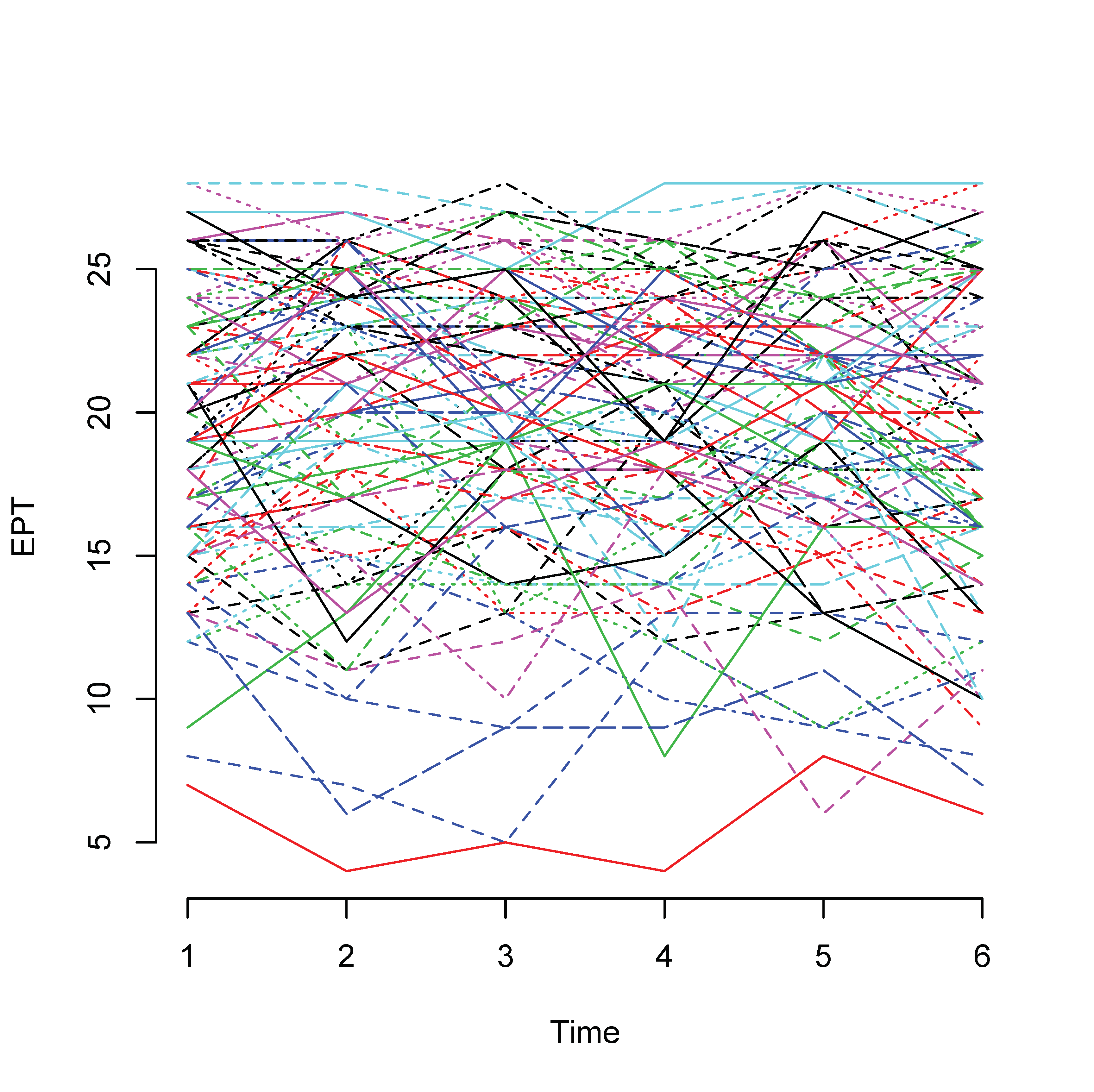
Longitudinal Data Analysis

Longitudinal data can be viewed as a special case of the multilevel data where time is nested within individual participants. All longitudinal data share at least three features: (1) the same entities are repeatedly observed over time; (2) the same measurements (including parallel tests) are used; and (3) the timing for each measurement is known (Baltes & Nesselroade, 1979). To study phenomena in their time-related patterns of constancy and change is a primary reason for collecting longitudinal data. Figure 1 show the plot of 50 participants from the ACTIVE study on the variable EPT for 6 times. Clearly, each line represents a participant. From it, we can see how an individual changes over time.

Growth curve model

Growth curve models (GCM; e.g., McArdle \& Nesselroade, 2003; Meredith & Tisak, 1990) exemplify a widely used technique with a direct match to the objectives of longitudinal research described by Baltes and Nesselroade (1979) to analyze explicitly intra-individual change and inter-individual differences in change. In the past decades, growth curve models have evolved from fitting a single curve for only one individual to fitting multilevel or mixed-effects models and from linear to nonlinear models (e.g., McArdle, 2001; McArdle & Nesselroade, 2003; Meredith & Tisak, 1990; Tucker, 1958; Wishart, 1938).

A typical linear growth curve model can be written as

\begin{eqnarray*} y_{it} & = & \beta_{0i}+\beta_{1i}\times time_{it}+e_{it}\\ \beta_{0i} & = & \gamma_{0}+v_{0i}\\ \beta_{1i} & = & \gamma_{1}+v_{1i}\end{eqnarray*}

where $y_{it}$ is data for participant $i$ at time $t$. For each individual $i$, a linear regression model can be fitted with its own intercept $\beta_{0i}$ and slope $\beta_{1i}$. On average, there is an intercept $\gamma_{0}$ and slope $\gamma_{1}$ for all individuals. The variation of $\beta_{0i}$ and $\beta_{1i}$ represents individual differences.

Individual difference can be further explained by other factors, for example, education level and age. Then the model is

\begin{eqnarray*} y_{it} & = & \beta_{0i}+\beta_{1i}\times time_{it}+e_{it}\\ \beta_{0i} & = & \gamma_{0}+\gamma_{1}\times edu_{i}+v_{0i}\\ \beta_{1i} & = & \gamma_{2}+\gamma_{3}\times edu_{i}+v_{1i} \end{eqnarray*}

GCM as a mulitlevel/mixed-effect model

A GCM can first be fitted as a multilevel model or mixed-effects model using the python library statsmodels.

To use the library, we would need to rewrite the growth curve model as a mixed-effect model, like in multilevel regression. For the model without second level predictor, we have

\begin{equation} y_{it}=\gamma_{0}+v_{i0}+\gamma_{1}*time_{it}+v_{1i}*time_{it}+e_{it}. \end{equation}

For the one with the second level predictor, such as education, we have

\begin{equation} y_{it}=\gamma_{0}+\gamma_{1}*edu+v_{0i}+\gamma_{2}*time_{it} +\gamma_{3}*edu_{i}*time_{it}+v_{1i}*time_{it}+e_{it}.\end{equation}

For demonstration, we investigate the growth of word set test (ws in the ACTIVE data set). In the current data set, we have the data in wide format, in which the 6 measures of ws are 6 variables. To use the python library, long format data are needed. For the long-format data, we need to stack the data from all waves into a long variable. The python code below reformats the data and plot them.

>>> import numpy as np
>>> ## data
>>> import pandas as pd
>>> active = pd.read_csv('https://advstats.psychstat.org/data/active.full.csv')
>>> 
>>> ## reshape the data to long format
>>> df_long = pd.melt(active, id_vars=['edu'], 
...                   value_vars=['ws1', 'ws2', 'ws3', 'ws4', 'ws5', 'ws6'],
...                   var_name='occ', value_name='score')
>>> df_long['time'] = np.repeat([1, 2, 3, 4, 5, 6], active.shape[0])
>>> df_long['id'] = np.tile(range(active.shape[0]), 6)
>>> df_long
      edu  occ  score  time    id
0      13  ws1      4     1     0
1      12  ws1     11     1     1
2      13  ws1      7     1     2
3      12  ws1     16     1     3
4      13  ws1      9     1     4
...   ...  ...    ...   ...   ...
6679   12  ws6     21     6  1109
6680   12  ws6     13     6  1110
6681   13  ws6     15     6  1111
6682   17  ws6     12     6  1112
6683   13  ws6      3     6  1113

[6684 rows x 5 columns]
>>> 
>>> import matplotlib.pyplot as plt
>>> import seaborn as sns
>>> ## plot
>>> sns.lineplot(data=df_long, x="occ", y="score", hue="id", legend=False)

>>> 
>>> plt.xlabel('Time')
Text(0.5, 0, 'Time')
>>> plt.ylabel('Reasoning')
Text(0, 0.5, 'Reasoning')
>>> 
>>> plt.savefig('long.svg', format='svg')
>>> plt.show()

Unconditional model (model without second level predictors)

Fitting the model is actually straightforward once rewriting the model in the mixed-effects format as in Equation (1). \begin{equation*} y_{it}=\gamma_{0}+v_{i0}+\gamma_{1}*time_{it}+v_{1i}*time_{it}+e_{it}. \end{equation*} The input and output are given below. Based on the output, the fixed effects for time (.214, t-value=11.59) is significant, therefore, there is a linear growth trend. The average intercept is 11.93 and is also significant. 

>>> import numpy as np
>>> ## data
>>> import pandas as pd
>>> active = pd.read_csv('https://advstats.psychstat.org/data/active.full.csv')
>>> 
>>> ## reshape the data to long format
>>> df_long = pd.melt(active, id_vars=['edu'], 
...                   value_vars=['ws1', 'ws2', 'ws3', 'ws4', 'ws5', 'ws6'],
...                   var_name='occ', value_name='score')
>>> df_long['time'] = np.repeat([1, 2, 3, 4, 5, 6], active.shape[0])
>>> df_long['id'] = np.tile(range(active.shape[0]), 6)
>>> df_long
      edu  occ  score  time    id
0      13  ws1      4     1     0
1      12  ws1     11     1     1
2      13  ws1      7     1     2
3      12  ws1     16     1     3
4      13  ws1      9     1     4
...   ...  ...    ...   ...   ...
6679   12  ws6     21     6  1109
6680   12  ws6     13     6  1110
6681   13  ws6     15     6  1111
6682   17  ws6     12     6  1112
6683   13  ws6      3     6  1113

[6684 rows x 5 columns]
>>> 
>>> ## use the statsmodels libray
>>> import statsmodels.api as sm
>>> import statsmodels.formula.api as smf
>>> 
>>> ## specify the model
>>> md = smf.mixedlm("score ~ time", 
...                  data=df_long, groups=df_long["id"],
...                  re_formula="~1 + time")
>>> 
>>> ## fit the model
>>> results = md.fit()
>>> 
>>> ## display the results
>>> print(results.summary())
           Mixed Linear Model Regression Results
===========================================================
Model:              MixedLM Dependent Variable: score      
No. Observations:   6684    Method:             REML       
No. Groups:         1114    Scale:              5.3609     
Min. group size:    6       Log-Likelihood:     -17044.1509
Max. group size:    6       Converged:          Yes        
Mean group size:    6.0                                    
-----------------------------------------------------------
                 Coef.  Std.Err.   z    P>|z| [0.025 0.975]
-----------------------------------------------------------
Intercept        11.926    0.152 78.424 0.000 11.628 12.224
time              0.214    0.018 11.590 0.000  0.178  0.250
Group Var        21.115    0.527                           
Group x time Cov  0.181    0.043                           
time Var          0.074    0.008                           
===========================================================

It is useful to test whether random-effects parameters such as the variances of intercept and slope are significance or not to evaluate individual differences. This can be done by comparing the current model with a model without random intercept or slope. The method is likelihood ratio test.

For example, to test the individual differences in slope for time. The random effects for time is .07. Based on the difference in the likelihood, which follows a chi-squared distribution, it is significant with p-value about 0. Therefore, there is significant individual difference in the growth rate (slope). This indicates that everyone has a different change rate. Note that in the alternative model m2, the random effect for time was not used.

>>> import numpy as np
>>> ## data
>>> import pandas as pd
>>> active = pd.read_csv('https://advstats.psychstat.org/data/active.full.csv')
>>> 
>>> ## reshape the data to long format
>>> df_long = pd.melt(active, id_vars=['edu'], 
...                   value_vars=['ws1', 'ws2', 'ws3', 'ws4', 'ws5', 'ws6'],
...                   var_name='occ', value_name='score')
>>> df_long['time'] = np.repeat([1, 2, 3, 4, 5, 6], active.shape[0])
>>> df_long['id'] = np.tile(range(active.shape[0]), 6)
>>> #df_long
>>> 
>>> ## use the statsmodels libray
>>> import statsmodels.api as sm
>>> import statsmodels.formula.api as smf
>>> 
>>> ## specify the model with both covariance
>>> m1 = smf.mixedlm("score ~ time", 
...                  data=df_long, groups=df_long["id"],
...                  re_formula="~1 + time")
>>> 
>>> ## fit the model
>>> results1 = m1.fit()
>>> 
>>> ## display the results
>>> print(results1.summary())
           Mixed Linear Model Regression Results
===========================================================
Model:              MixedLM Dependent Variable: score      
No. Observations:   6684    Method:             REML       
No. Groups:         1114    Scale:              5.3609     
Min. group size:    6       Log-Likelihood:     -17044.1509
Max. group size:    6       Converged:          Yes        
Mean group size:    6.0                                    
-----------------------------------------------------------
                 Coef.  Std.Err.   z    P>|z| [0.025 0.975]
-----------------------------------------------------------
Intercept        11.926    0.152 78.424 0.000 11.628 12.224
time              0.214    0.018 11.590 0.000  0.178  0.250
Group Var        21.115    0.527                           
Group x time Cov  0.181    0.043                           
time Var          0.074    0.008                           
===========================================================

>>> 
>>> ## specify an alternative model
>>> m2 = smf.mixedlm("score ~ time", 
...                  data=df_long, groups=df_long["id"],
...                  re_formula="~1")
>>> 
>>> ## fit the model
>>> results2 = m2.fit()
>>> 
>>> ## display the results
>>> print(results2.summary())
          Mixed Linear Model Regression Results
=========================================================
Model:            MixedLM Dependent Variable: score      
No. Observations: 6684    Method:             REML       
No. Groups:       1114    Scale:              5.6185     
Min. group size:  6       Log-Likelihood:     -17066.7246
Max. group size:  6       Converged:          Yes        
Mean group size:  6.0                                    
----------------------------------------------------------
           Coef.   Std.Err.    z     P>|z|  [0.025  0.975]
----------------------------------------------------------
Intercept  11.926     0.159  75.075  0.000  11.615  12.237
time        0.214     0.017  12.609  0.000   0.181   0.247
Group Var  23.241     0.474                               
=========================================================

>>> 
>>> ## difference in the likilihood
>>> delta_ll = -2*(results2.llf - results1.llf)
>>> delta_ll
np.float64(45.14731834300619)
>>> 
>>> delta_df = 2
>>> 
>>> ## get the p-value
>>> from scipy.stats import chi2
>>> 1 - chi2.cdf(delta_ll, delta_df)
np.float64(1.5717538381920804e-10)

To test the individual differences in intercept. The random effects for intercept is 21.11. Based on ANOVA analysis below, it is significant. Therefore, there is individual difference or individuals have different intercepts.

>>> import numpy as np
>>> ## data
>>> import pandas as pd
>>> active = pd.read_csv('https://advstats.psychstat.org/data/active.full.csv')
>>> 
>>> ## reshape the data to long format
>>> df_long = pd.melt(active, id_vars=['edu'], 
...                   value_vars=['ws1', 'ws2', 'ws3', 'ws4', 'ws5', 'ws6'],
...                   var_name='occ', value_name='score')
>>> df_long['time'] = np.repeat([1, 2, 3, 4, 5, 6], active.shape[0])
>>> df_long['id'] = np.tile(range(active.shape[0]), 6)
>>> #df_long
>>> 
>>> ## use the statsmodels libray
>>> import statsmodels.api as sm
>>> import statsmodels.formula.api as smf
>>> 
>>> ## specify the model with both covariance
>>> m1 = smf.mixedlm("score ~ time", 
...                  data=df_long, groups=df_long["id"],
...                  re_formula="~1 + time")
>>> 
>>> ## fit the model
>>> results1 = m1.fit()
>>> 
>>> ## display the results
>>> print(results1.summary())
           Mixed Linear Model Regression Results
===========================================================
Model:              MixedLM Dependent Variable: score      
No. Observations:   6684    Method:             REML       
No. Groups:         1114    Scale:              5.3609     
Min. group size:    6       Log-Likelihood:     -17044.1509
Max. group size:    6       Converged:          Yes        
Mean group size:    6.0                                    
-----------------------------------------------------------
                 Coef.  Std.Err.   z    P>|z| [0.025 0.975]
-----------------------------------------------------------
Intercept        11.926    0.152 78.424 0.000 11.628 12.224
time              0.214    0.018 11.590 0.000  0.178  0.250
Group Var        21.115    0.527                           
Group x time Cov  0.181    0.043                           
time Var          0.074    0.008                           
===========================================================

>>> 
>>> ## specify an alternative model
>>> m2 = smf.mixedlm("score ~ time", 
...                  data=df_long, groups=df_long["id"],
...                  re_formula="~ 0 + time")
>>> 
>>> ## fit the model
>>> results2 = m2.fit()
>>> 
>>> ## display the results
>>> print(results2.summary())
          Mixed Linear Model Regression Results
=========================================================
Model:            MixedLM Dependent Variable: score      
No. Observations: 6684    Method:             REML       
No. Groups:       1114    Scale:              10.2300    
Min. group size:  6       Log-Likelihood:     -18639.0075
Max. group size:  6       Converged:          Yes        
Mean group size:  6.0                                    
---------------------------------------------------------
              Coef.  Std.Err.    z    P>|z| [0.025 0.975]
---------------------------------------------------------
Intercept     11.926    0.089 133.680 0.000 11.751 12.101
time           0.214    0.040   5.306 0.000  0.135  0.293
time Var       1.228    0.019                            
=========================================================

>>> 
>>> ## difference in the likilihood
>>> delta_ll = -2*(results2.llf - results1.llf)
>>> delta_ll
np.float64(3189.7131050783937)
>>> 
>>> delta_df = 2
>>> 
>>> ## get the p-value
>>> from scipy.stats import chi2
>>> 1 - chi2.cdf(delta_ll, delta_df)
np.float64(0.0)

Conditional model (model with second level predictors)

Using the same set of data, we now investigate whether education is a predictor of random intercept and slope. The model is given below: \begin{equation} y_{it}=\gamma_{0}+\gamma_{1}*edu+v_{0i}+\gamma_{2}*time_{it} +\gamma_{3}*edu_{i}*time_{it}+v_{1i}*time_{it}+e_{it}.\end{equation} Given there is individual differences in intercept and slope, we want to explain why. So, we use Edu as a explanatory variable. From the output, we can see that the parameter \(\gamma_{1} = .78\) is significant. Higher education relates to bigger intercept. In addition, the parameter $\gamma_{3} = -.022$ is significant. Higher education relates to lower growth rate of ws.

>>> import numpy as np
>>> ## data
>>> import pandas as pd
>>> active = pd.read_csv('https://advstats.psychstat.org/data/active.full.csv')
>>> 
>>> ## reshape the data to long format
>>> df_long = pd.melt(active, id_vars=['edu'], 
...                   value_vars=['ws1', 'ws2', 'ws3', 'ws4', 'ws5', 'ws6'],
...                   var_name='occ', value_name='score')
>>> df_long['time'] = np.repeat([1, 2, 3, 4, 5, 6], active.shape[0])
>>> df_long['id'] = np.tile(range(active.shape[0]), 6)
>>> df_long
      edu  occ  score  time    id
0      13  ws1      4     1     0
1      12  ws1     11     1     1
2      13  ws1      7     1     2
3      12  ws1     16     1     3
4      13  ws1      9     1     4
...   ...  ...    ...   ...   ...
6679   12  ws6     21     6  1109
6680   12  ws6     13     6  1110
6681   13  ws6     15     6  1111
6682   17  ws6     12     6  1112
6683   13  ws6      3     6  1113

[6684 rows x 5 columns]
>>> 
>>> ## use the statsmodels libray
>>> import statsmodels.api as sm
>>> import statsmodels.formula.api as smf
>>> 
>>> ## specify the model
>>> md = smf.mixedlm("score ~ time + edu + time*edu", 
...                  data=df_long, groups=df_long["id"],
...                  re_formula="~1 + time")
>>> 
>>> ## fit the model
>>> results = md.fit()
>>> 
>>> ## display the results
>>> print(results.summary())
           Mixed Linear Model Regression Results
===========================================================
Model:              MixedLM Dependent Variable: score      
No. Observations:   6684    Method:             REML       
No. Groups:         1114    Scale:              5.5542     
Min. group size:    6       Log-Likelihood:     -16960.1403
Max. group size:    6       Converged:          Yes        
Mean group size:    6.0                                    
-----------------------------------------------------------
                 Coef.  Std.Err.   z    P>|z| [0.025 0.975]
-----------------------------------------------------------
Intercept         1.240    0.741  1.674 0.094 -0.212  2.692
time              0.528    0.093  5.676 0.000  0.345  0.710
edu               0.778    0.053 14.679 0.000  0.674  0.882
time:edu         -0.023    0.007 -3.433 0.001 -0.036 -0.010
Group Var        16.316    0.416                           
Group x time Cov  0.497    0.032                           
time Var          0.015    0.006                           
===========================================================

GCM as a SEM

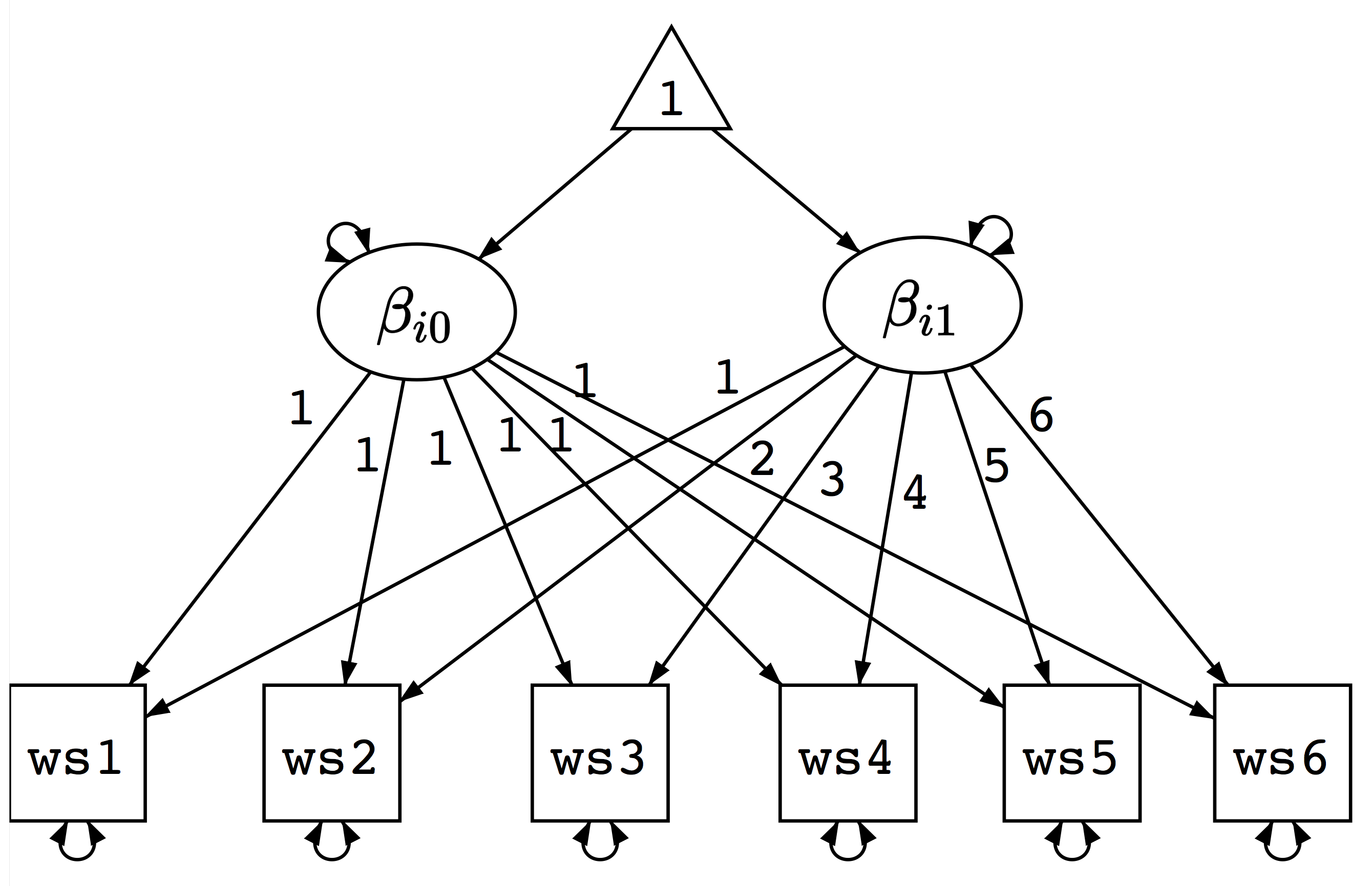
In addition to estimating a GCM as a multilevel or mixed-effects model, we can also estimate it as a SEM. To illustrate this, we consider a linear growth curve model. If a group of participants all have linear change trend, for each individual, we can fit a regression model such as \[ y_{it}=\beta_{i0}+\beta_{i1}t+e_{it} \] where $\beta_{i0}$ and $\beta_{i1}$ are intercept and slope, respectively. Note that here we let $time_{it} = t$. If each individual has different time of data collection, it can still be done in the SEM framework but would be more complex. By writing the time out, we would have \[ \left(\begin{array}{c} y_{i1}\\ y_{i2}\\ \vdots\\ y_{iT} \end{array}\right)=\left(\begin{array}{cc} 1 & 1\\ 1 & 2\\ 1 & \vdots\\ 1 & T \end{array}\right)\left(\begin{array}{c} \beta_{i0}\\ \beta_{i1} \end{array}\right)+\left(\begin{array}{c} e_{i1}\\ e_{i2}\\ \vdots\\ e_{iT} \end{array}\right) \]

Note that the above equation resembles a factor model with two factors - $b_{0}$ and $b_{1}$ and a factor loading matrix with known factor loading matrix. The individual intercept and slope can be viewed as factor scores to be estimated. Furthermore, we are interested in model with mean structure because the means of $\beta_{0}$ and $\beta_{1}$ have their meaning as average intercept and slope (rate of change). The variances of the factors can be estimated - they indicate the variations of intercept and slope. Using path diagram, the model is shown in the figure below.

With the model, we can estimate it using the semopy package. Unlike the statsmodels package, in using SEM, the wide format of data is directly used. The python input and output for the unconditional model is given below.

Using this method, each parameter in the model can be directly tested using a z-test. In addition, we can use the fit statistics for SEM to test the fit of the growth curve model. Note the fit statistics from semopy need to be evaluated first before using.

Note that to specify the mean structure, we use ~1 to indicate the mean of the factor. For example, to specify the mean for the level factor, we use level ~ 1. At the time of writing (Nov 30, 2024), there is bug with the starting values for the latent factor means. Therefore, we need to specify the starting values for the latent factor means. To do it, we use code like below

level ~ a*1
slope ~ b*1

START(12.0) a
START(0.16) b

>>> import pandas as pd
>>> import semopy as sem
>>> 
>>> active = pd.read_csv('https://advstats.psychstat.org/data/active.full.csv')
>>> active.head()
   group  training  gender  age  edu  mmse  ...  ept5  hvltt6  ws6  ls6  lt6  ept6
0      3         1       2   67   13    27  ...    24      23    8   12    6    21
1      4         0       2   69   12    28  ...    22      28   17   16    7    17
2      1         1       2   77   13    26  ...    21      18   10   13    6    20
3      4         0       2   79   12    30  ...     9      21   12   14    6    11
4      4         0       2   78   13    27  ...    14      19    4    7    3    16

[5 rows x 36 columns]
>>> 
>>> # Define the path model using the function Model
>>> gcm = '''
...     level =~ 1*ws1 + 1*ws2 + 1*ws3 + 1*ws4 + 1*ws5 + 1*ws6
...     slope =~ 1*ws1 + 2*ws2 + 3*ws3 + 4*ws4 + 5*ws5 + 6*ws6
...     level ~~ level
...     slope ~~ slope
...     level ~~ slope
...     level ~ 1
...     slope ~ 1
...     ws1 ~ 0*1
...     ws2 ~ 0*1
...     ws3 ~ 0*1
...     ws4 ~ 0*1
...     ws5 ~ 0*1
...     ws6 ~ 0*1
... '''
>>> 
>>> # Create the SEM model
>>> model = sem.Model(gcm)
>>> 
>>> # Fit the model to data
>>> model.fit(active)
>>> 
>>> # Get parameter estimates and model fit statistics
>>> params = model.inspect()
>>> print(params)
     lval  op   rval       Estimate Std. Err z-value p-value
0   level   ~      1  Not estimated        -       -       -
1   slope   ~      1  Not estimated        -       -       -
2     ws1   ~  level            1.0        -       -       -
3     ws1   ~  slope            1.0        -       -       -
4     ws2   ~  level            1.0        -       -       -
5     ws2   ~  slope            2.0        -       -       -
6     ws3   ~  level            1.0        -       -       -
7     ws3   ~  slope            3.0        -       -       -
8     ws4   ~  level            1.0        -       -       -
9     ws4   ~  slope            4.0        -       -       -
10    ws5   ~  level            1.0        -       -       -
11    ws5   ~  slope            5.0        -       -       -
12    ws6   ~  level            1.0        -       -       -
13    ws6   ~  slope            6.0        -       -       -
14    ws1   ~      1            0.0        -       -       -
15    ws2   ~      1            0.0        -       -       -
16    ws3   ~      1            0.0        -       -       -
17    ws4   ~      1            0.0        -       -       -
18    ws5   ~      1            0.0        -       -       -
19    ws6   ~      1            0.0        -       -       -
20  level  ~~  level  Not estimated        -       -       -
21  level  ~~  slope  Not estimated        -       -       -
22  slope  ~~  slope  Not estimated        -       -       -
23    ws1  ~~    ws1  Not estimated        -       -       -
24    ws2  ~~    ws2  Not estimated        -       -       -
25    ws3  ~~    ws3  Not estimated        -       -       -
26    ws4  ~~    ws4  Not estimated        -       -       -
27    ws5  ~~    ws5  Not estimated        -       -       -
28    ws6  ~~    ws6  Not estimated        -       -       -
>>> 
>>> # Check model fit
>>> fit_stats = sem.calc_stats(model)
>>> print(fit_stats.T)

Fitting a conditional model is similar but one would need to use the predictor for the factors. 

>>> import pandas as pd
>>> import semopy as sem
>>> 
>>> active = pd.read_csv('https://advstats.psychstat.org/data/active.full.csv')
>>> active.head()
   group  training  gender  age  edu  mmse  ...  ept5  hvltt6  ws6  ls6  lt6  ept6
0      3         1       2   67   13    27  ...    24      23    8   12    6    21
1      4         0       2   69   12    28  ...    22      28   17   16    7    17
2      1         1       2   77   13    26  ...    21      18   10   13    6    20
3      4         0       2   79   12    30  ...     9      21   12   14    6    11
4      4         0       2   78   13    27  ...    14      19    4    7    3    16

[5 rows x 36 columns]
>>> 
>>> # Define the path model using the function Model
>>> gcm = '''
...     level =~ 1*ws1 + 1*ws2 + 1*ws3 + 1*ws4 + 1*ws5 + 1*ws6
...     slope =~ 1*ws1 + 2*ws2 + 3*ws3 + 4*ws4 + 5*ws5 + 6*ws6
...     level ~~ level
...     slope ~~ slope
...     level ~~ slope
...     level ~ a*1 + edu
...     slope ~ b*1 + edu
...     ws1 ~ 0*1
...     ws2 ~ 0*1
...     ws3 ~ 0*1
...     ws4 ~ 0*1
...     ws5 ~ 0*1
...     ws6 ~ 0*1
...     START(12.0) a
...     START(0.16) b
... '''
>>> 
>>> # Create the SEM model
>>> model = sem.ModelMeans(gcm)
>>> 
>>> # Fit the model to data
>>> model.fit(active)
SolverResult(fun=np.float64(21444.94012083019), success=np.True_, n_it=39, x=array([16.74038823,  0.51395716,  0.        ,  8.81471105,  5.61811118,
        3.90064823,  4.0918114 ,  4.69873705,  6.38537143,  1.50940699,
        0.78181375,  0.48591184, -0.02347183]), message='Optimization terminated successfully', name_method='SLSQP', name_obj='FIML')
>>> 
>>> # Get parameter estimates and model fit statistics
>>> params = model.inspect()
>>> print(params)
     lval  op   rval   Estimate  Std. Err    z-value   p-value
0   level   ~    edu   0.781814  0.054734  14.283896       0.0
1   slope   ~    edu  -0.023472  0.007053  -3.327982  0.000875
2     ws1   ~  level   1.000000         -          -         -
3     ws1   ~  slope   1.000000         -          -         -
4     ws2   ~  level   1.000000         -          -         -
5     ws2   ~  slope   2.000000         -          -         -
6     ws3   ~  level   1.000000         -          -         -
7     ws3   ~  slope   3.000000         -          -         -
8     ws4   ~  level   1.000000         -          -         -
9     ws4   ~  slope   4.000000         -          -         -
10    ws5   ~  level   1.000000         -          -         -
11    ws5   ~  slope   5.000000         -          -         -
12    ws6   ~  level   1.000000         -          -         -
13    ws6   ~  slope   6.000000         -          -         -
14  level   ~      1   1.509407  0.765216   1.972524   0.04855
15  slope   ~      1   0.485912  0.098604   4.927924  0.000001
16    ws1   ~      1   0.000000         -          -         -
17    ws2   ~      1   0.000000         -          -         -
18    ws3   ~      1   0.000000         -          -         -
19    ws4   ~      1   0.000000         -          -         -
20    ws5   ~      1   0.000000         -          -         -
21    ws6   ~      1   0.000000         -          -         -
22  level  ~~  level  16.740388  0.968841  17.278785       0.0
23  level  ~~  slope   0.513957  0.098492   5.218289       0.0
24  slope  ~~  slope   0.000000  0.019035        0.0       1.0
25    ws1  ~~    ws1   8.814711  0.433655  20.326548       0.0
26    ws2  ~~    ws2   5.618111   0.28255   19.88361       0.0
27    ws3  ~~    ws3   3.900648  0.208799  18.681345       0.0
28    ws4  ~~    ws4   4.091811  0.219422  18.648145       0.0
29    ws5  ~~    ws5   4.698737  0.248989  18.871257       0.0
30    ws6  ~~    ws6   6.385371  0.341913  18.675422       0.0
>>> 
>>> # Check model fit
>>> fit_stats = sem.calc_stats(model)
>>> print(fit_stats.T)
                   Value
DoF             8.000000
DoF Baseline   13.000000
chi2           19.250395
chi2 p-value    0.013576
chi2 Baseline  37.425897
CFI             0.539407
GFI             0.485640
AGFI            0.164165
NFI             0.485640
TLI             0.251537
RMSEA           0.035546
AIC            25.728427
BIC            90.932688
LogLik          0.135787