
Path Analysis
Path analysis is a type of statistical method to investigate the direct and indirect relationship among a set of exogenous (independent, predictor, input) and endogenous (dependent, output) variables. Path analysis can be viewed as generalization of regression and mediation analysis where multiple input, mediators, and output can be used. The purpose of path analysis is to study relationships among a set of observed variables, e.g., estimate and test direct and indirect effects in a system of regression equations and estimate and test theories about the absence of relationships
Path diagrams
Path analysis is often conducted based on path diagrams. Path diagram represents a model using shapes and paths. For example, the diagram below portrays the multiple regression model $Y=\beta_0 + \beta_X X + \beta_W W + \beta_Z Z + e$.
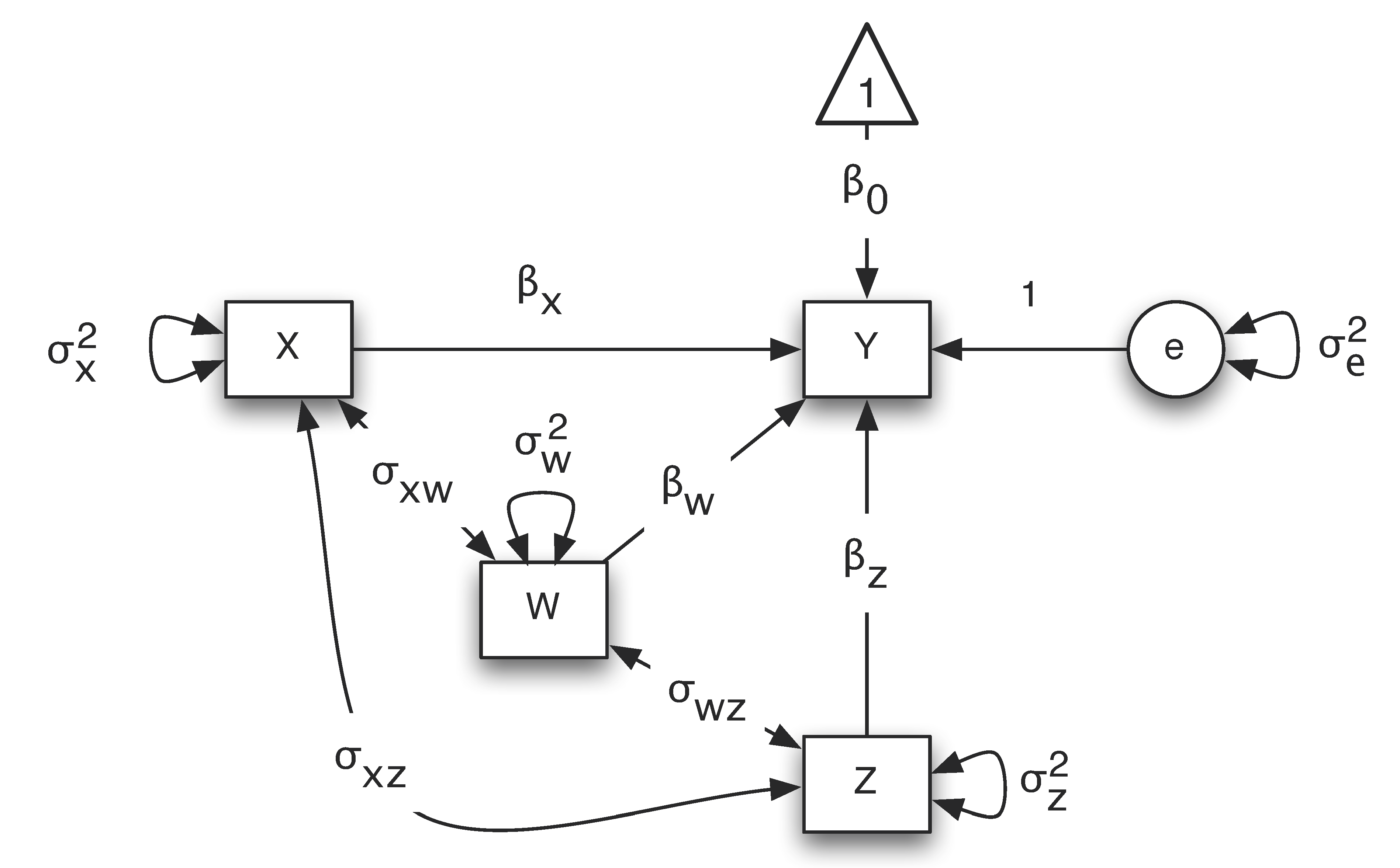
In a path diagram, different shapes and paths have different meanings:
- Squares or rectangular boxes: observed or manifest variables
- Circles or ovals: errors, factors, latent variables
- Single-headed arrows: linear relationship between two variables. Starts from an independent variable and ends on a dependent variable.
- Double-headed arrows: variance of a variable or covariance between two variables
- Triangle: a constant variable, usually a vector of ones
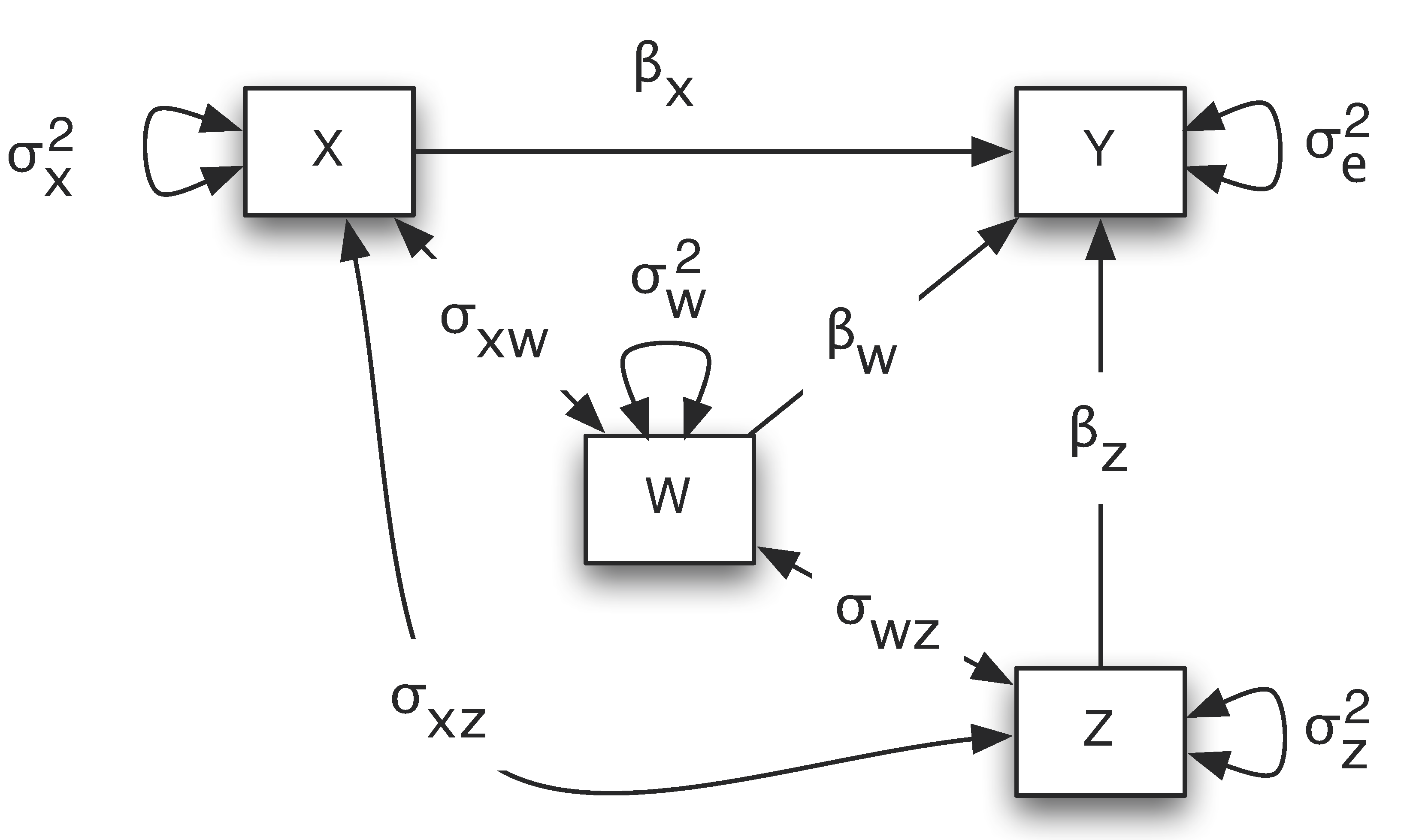
A simplified path diagram is often used in practice in which the intercept term is removed and the residual variances are directly put on the outcome variables. For example, for the regression example, the path diagram is shown below.
In python, path analysis can be conducted using the Python library semopy. semopy stands for Structural Equation Models Optimization in Python and is a powerful statistical technique that combines elements of regression, factor analysis, and path analysis to analyze relationships between observed (measured) and latent (unobserved) variables. The library is designed to be user-friendly and easy to use. It provides a simple interface to specify a model and estimate the parameters. The library also provides a variety of tools to evaluate the model fit, such as the chi-square test, RMSEA, CFI, and TLI.
We now show how to conduct path analysis using several examples.
Example 1. Mediation analysis -- Test the direct and indirect effects
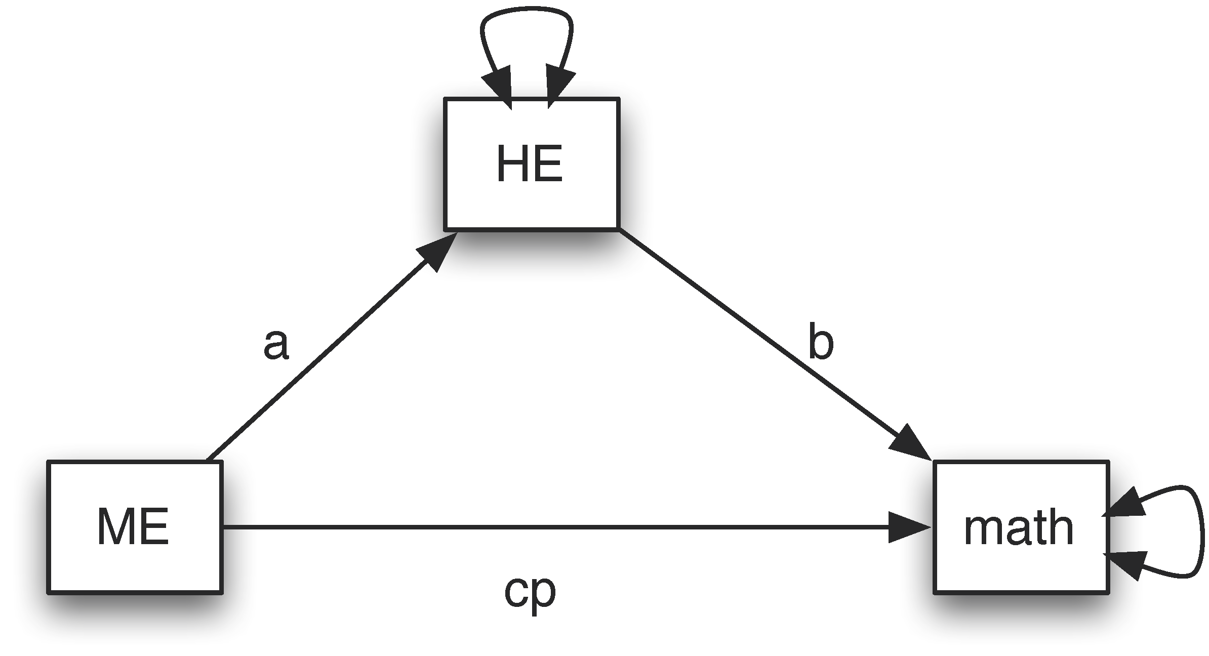
The NLSY data include three variables – mother's education (ME), home environment (HE), and child's math score. Assume we want to test whether home environment is a mediator between mother’s education and child's math score. The path diagram for the mediation model is:
To estimate the paths in the model, we use the Python library semopy. To specify the mediation model, we follow the rules below. First, a model can be specified using strings. The triple-quoted strings, which are strings enclosed in three single quotes (''') or three double quotes (""") are used. The quotes surround a model. Second, to specify the regression relationship, we use a symbol ~. The variable on the left is the outcome and the ones on the right are predictors or covariates. Third, to specify the covariance relationship, we use a symbol ~~. Fourth, parameter names can be used for paths in model specification such as a, b and cp.
With the specified model in string, we can compile is using the Model() function. The fit() function is used to estimate the parameters. The inspect() function is used to get the parameter estimates. To get the fit statistics, the calc_stats() function is used. For example, for the mediation example, the input and output are given below.
>>> import pandas as pd
>>> import semopy as sem
>>>
>>> nlsy = pd.read_csv('https://advstats.psychstat.org/data/nlsy.csv')
>>> nlsy.head()
   ME  HE  math
0  12   6     6
1  15   6    11
2   9   5     3
3   8   3     6
4   9   6    11
>>>
>>> # Define the path model using the function Model
>>> med = '''
...     math ~ HE + ME
...     HE ~ ME
...     ME ~~ ME
... '''
>>>
>>> # Create the SEM model
>>> model = sem.Model(med)
>>>
>>> # Fit the model to data
>>> model.fit(nlsy)
SolverResult(fun=np.float64(8.785567562341612e-08), success=True, n_it=19, x=array([ 0.46453692,  0.46244455,  0.1391007 ,  3.9951032 ,  2.72321485,
       20.61697808]), message='Optimization terminated successfully', name_method='SLSQP', name_obj='MLW')
>>>
>>> # Get parameter estimates and model fit statistics
>>> params = model.inspect()
>>> print(params)
   lval  op  rval   Estimate  Std. Err    z-value   p-value
0    HE   ~    ME   0.139101  0.042864   3.245184  0.001174
1  math   ~    HE   0.464537  0.142851   3.251888  0.001146
2  math   ~    ME   0.462445  0.119602   3.866518  0.000110
3    ME  ~~    ME   3.995103  0.293330  13.619838  0.000000
4    HE  ~~    HE   2.723215  0.199945  13.619838  0.000000
5  math  ~~  math  20.616978  1.513746  13.619838  0.000000
>>>
>>> # Check model fit
>>> fit_stats = sem.calc_stats(model)
>>> print(fit_stats.T)
                      Value
DoF            0.000000e+00
DoF Baseline   3.000000e+00
chi2           3.259446e-05
chi2 p-value            NaN
chi2 Baseline  3.978475e+01
CFI            9.999991e-01
GFI            9.999992e-01
AGFI                    NaN
NFI            9.999992e-01
TLI                     NaN
RMSEA                   inf
AIC            1.200000e+01
BIC            3.549721e+01
LogLik         8.785568e-08
>>>
>>> # mediation effect
>>> print(params.loc[0, 'Estimate'] * params.loc[1, 'Estimate'])
0.06461740868004863
>>>
>>> # plot the model
>>> # sem.semplot(med, 'mediation0.svg') ## without coefficients
>>> sem.semplot(model, 'mediation.svg')  ## with coefficients
- An individual path can be tested. For example, the coefficient from ME to HE is 0.139, which is significant based on the z-test.
- The residual variance parameters are also automatically estimated.
The mediation effect can be calculated using the parameter estimates. The mediation effect is the product of the path from ME to HE and the path from HE to math. For testing the effect, we will use the bootstrap method.
Example 2. Testing a theory of no direct effect
Assume we hypothesize that there is no direct effect from ME to math. To test the hypothesis, we can fit a model illustrated below.
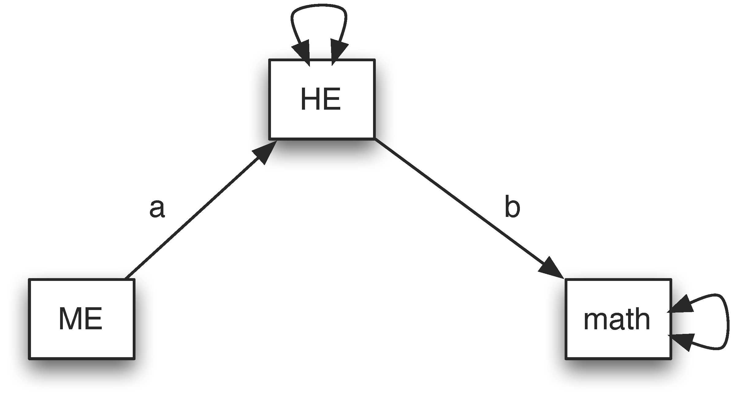
The input and output of the analysis are given below. To evaluate the hypothesis, we can check the model fit. The null hypothesis is “\(H_{0}\): The model fits the data well or the model is supported”. The alternative hypothesis is “\(H_{1}\): The model does not fit the data or the model is rejected”. The model with the direct effect fits the data perfectly. Therefore, if the current model also fits the data well, we fail to reject the null hypothesis. Otherwise, we reject it. The test of the model can be conducted based on a chi-squared test. From the output, the Chi-square is 14.676 with 1 degree of freedom. The p-value is about 0. Therefore, the null hypothesis is rejected. This indicates that the model without direct effect is not a good model.
>>> import pandas as pd
>>> import semopy as sem
>>>
>>> nlsy = pd.read_csv('https://advstats.psychstat.org/data/nlsy.csv')
>>> nlsy.head()
   ME  HE  math
0  12   6     6
1  15   6    11
2   9   5     3
3   8   3     6
4   9   6    11
>>>
>>> # Define the path model using the function Model
>>> med = '''
...     math ~ HE
...     HE ~ ME
...     ME ~~ ME
... '''
>>>
>>> # Create the SEM model
>>> model = sem.Model(med)
>>>
>>> # Fit the model to data
>>> model.fit(nlsy)
SolverResult(fun=np.float64(0.039558178472407945), success=True, n_it=19, x=array([ 0.55679084,  0.13915528,  3.9951032 ,  2.72351785, 21.45130121]), message='Optimization terminated successfully', name_method='SLSQP', name_obj='MLW')
>>>
>>> # Get parameter estimates and model fit statistics
>>> params = model.inspect()
>>> print(params)
   lval  op  rval   Estimate  Std. Err    z-value   p-value
0    HE   ~    ME   0.139155  0.042866   3.246277  0.001169
1  math   ~    HE   0.556791  0.143679   3.875248  0.000107
2    ME  ~~    ME   3.995103  0.293330  13.619838  0.000000
3    HE  ~~    HE   2.723518  0.199967  13.619838  0.000000
4  math  ~~  math  21.451301  1.575004  13.619838  0.000000
>>>
>>> # Check model fit
>>> fit_stats = sem.calc_stats(model)
>>> print(fit_stats.T)
                   Value
DoF             1.000000
DoF Baseline    3.000000
chi2           14.676084
chi2 p-value    0.000128
chi2 Baseline  39.784755
CFI             0.628213
GFI             0.631113
AGFI           -0.106661
NFI             0.631113
TLI            -0.115360
RMSEA           0.192256
AIC             9.920884
BIC            29.501894
LogLik          0.039558
Example 3: A more complex path model
Path analysis can be used to test more complex theories. In this example, we look at how age and education influence EPT using the ACTIVE data. Both age and education may influence EPT directly or through memory and reasoning ability. Therefore, we can fit a model shown below.
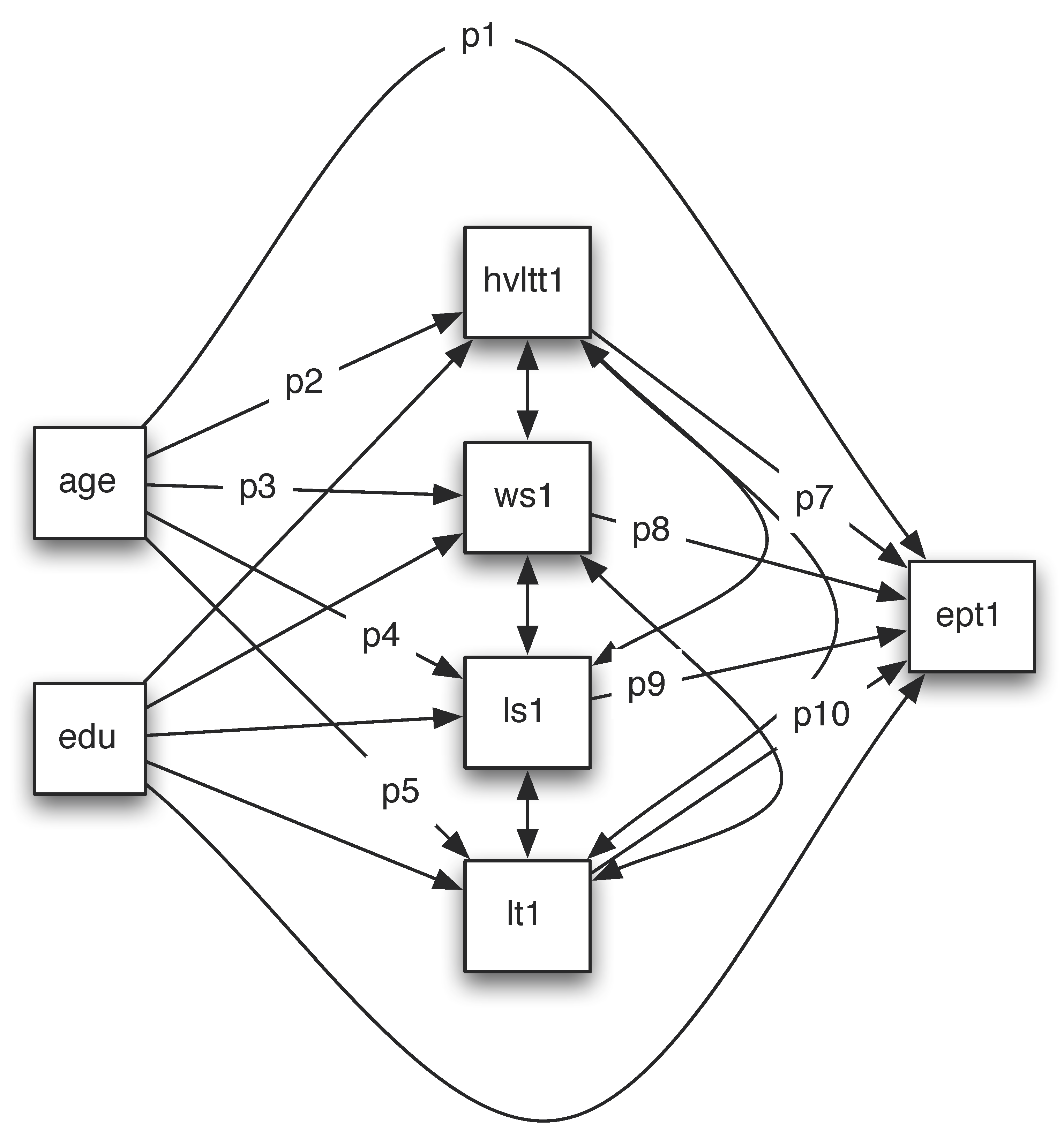
Suppose we want to test the total effect of age on EPT and its indirect effect. The direct effect is the path from age to ept1 directly, denoted by p1. One indirect path goes through hvltt1, that is p2*p7. The second indirect effect through ws1 is p3*p8. The third indirect effect through ls1 is p4*p9. The last indirect effect through lt1 is p5*p10. The total indirect effect is p2*p7+p3*p8+p4*p9+p5*p10. The total effect is the sum of them p1+p2*p7+p3*p8+p4*p9+p5*p10.
The output from such a model is given below. From it, we can see that the indirect effect ind1=p2*p7 is significant. The total indirect (indirect) from age to EPT is also significant. Finally, the total effect (total) from age to EPT is significant.
>>> import pandas as pd
>>> import semopy as sem
>>>
>>> active = pd.read_csv('https://advstats.psychstat.org/data/active.full.csv')
>>> active.head()
   group  training  gender  age  edu  mmse  ...  ept5  hvltt6  ws6  ls6  lt6  ept6
0      3         1       2   67   13    27  ...    24      23    8   12    6    21
1      4         0       2   69   12    28  ...    22      28   17   16    7    17
2      1         1       2   77   13    26  ...    21      18   10   13    6    20
3      4         0       2   79   12    30  ...     9      21   12   14    6    11
4      4         0       2   78   13    27  ...    14      19    4    7    3    16

[5 rows x 36 columns]
>>>
>>> # Define the path model using the function Model
>>> med = '''
...     hvltt1 ~ age + edu
...     ws1 ~ age + edu
...     ls1 ~ age + edu
...     lt1 ~ age + edu
...     ept1 ~ age + edu + hvltt1 + ws1 + ls1 + lt1
...     age ~~ age
...     edu ~~ edu
...     age ~~ edu
...     hvltt1 ~~ ws1 + ls1 + lt1
...     ws1 ~~ ls1 + lt1
...     ls1 ~~ lt1
... '''
>>>
>>> # Create the SEM model
>>> model = sem.Model(med)
>>>
>>> # Fit the model to data
>>> model.fit(active, obj='MLW')
SolverResult(fun=np.float64(2.696444668259801e-05), success=True, n_it=69, x=array([-1.60949969e-01,  4.29025011e-01, -2.25689229e-01,  7.04332936e-01,
       -2.76307048e-01,  8.77173999e-01, -8.54662686e-02,  3.94002008e-01,
        1.37129234e-02,  4.48298951e-01,  2.02464085e-01,  1.95712061e-01,
        2.45621990e-01,  1.50610194e-01,  2.64752022e+01, -9.19226170e-01,
        6.75398229e+00,  7.60103819e+00,  8.48481022e+00,  2.86800334e+00,
        2.06332206e+01,  1.65720608e+01,  5.70004236e+00,  1.95461570e+01,
        6.56166923e+00,  2.40035114e+01,  1.21075359e+01,  6.16833077e+00]), message='Optimization terminated successfully', name_method='SLSQP', name_obj='MLW')
>>>
>>> # Get parameter estimates and model fit statistics
>>> params = model.inspect()
>>> print(params)
      lval  op    rval   Estimate  Std. Err    z-value       p-value
0   hvltt1   ~     age  -0.160950  0.026512  -6.070732  1.273284e-09
1   hvltt1   ~     edu   0.429025  0.052492   8.173218  2.220446e-16
2      ws1   ~     age  -0.225689  0.025805  -8.746088  0.000000e+00
3      ws1   ~     edu   0.704333  0.051090  13.786096  0.000000e+00
4      ls1   ~     age  -0.276307  0.028596  -9.662472  0.000000e+00
5      ls1   ~     edu   0.877174  0.056617  15.493244  0.000000e+00
6      lt1   ~     age  -0.085466  0.014496  -5.895825  3.728135e-09
7      lt1   ~     edu   0.394002  0.028701  13.728042  0.000000e+00
8     ept1   ~     age   0.013713  0.021229   0.645953  5.183095e-01
9     ept1   ~     edu   0.448299  0.045098   9.940634  0.000000e+00
10    ept1   ~  hvltt1   0.202464  0.025110   8.063206  6.661338e-16
11    ept1   ~     ws1   0.195712  0.037700   5.191269  2.088653e-07
12    ept1   ~     ls1   0.245622  0.034545   7.110133  1.159295e-12
13    ept1   ~     lt1   0.150610  0.050866   2.960923  3.067187e-03
14     age  ~~     age  26.475202  1.121790  23.600847  0.000000e+00
15     age  ~~     edu  -0.919226  0.401588  -2.288978  2.208062e-02
16     edu  ~~     edu   6.753982  0.286175  23.600847  0.000000e+00
17  hvltt1  ~~     ws1   7.601038  0.643345  11.814879  0.000000e+00
18  hvltt1  ~~     ls1   8.484810  0.713591  11.890305  0.000000e+00
19  hvltt1  ~~     lt1   2.868003  0.348758   8.223484  2.220446e-16
20  hvltt1  ~~  hvltt1  20.633221  0.874258  23.600847  0.000000e+00
21     ws1  ~~     ls1  16.572061  0.817125  20.280947  0.000000e+00
22     ws1  ~~     lt1   5.700042  0.370668  15.377763  0.000000e+00
23     ws1  ~~     ws1  19.546157  0.828197  23.600847  0.000000e+00
24     ls1  ~~     lt1   6.561669  0.414197  15.841896  0.000000e+00
25     ls1  ~~     ls1  24.003511  1.017061  23.600847  0.000000e+00
26     lt1  ~~     lt1   6.168331  0.261361  23.600847  0.000000e+00
27    ept1  ~~    ept1  12.107536  0.513013  23.600847  0.000000e+00
>>>
>>> # Check model fit
>>> fit_stats = sem.calc_stats(model)
>>> print(fit_stats.T)
                     Value
DoF               0.000000
DoF Baseline     21.000000
chi2              0.030038
chi2 p-value           NaN
chi2 Baseline  3349.940000
CFI               0.999991
GFI               0.999991
AGFI                   NaN
NFI               0.999991
TLI                    NaN
RMSEA                  inf
AIC              55.999946
BIC             196.439894
LogLik            0.000027
To cite the book, use:
Zhang, Z. & Wang, L. (2017-2026). Advanced statistics using R. Granger, IN: ISDSA Press. https://doi.org/10.35566/advstats. ISBN: 978-1-946728-01-2.
To take the full advantage of the book such as running analysis within your web browser, please subscribe.